Plant Components
Heat Exchanger
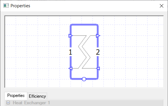
The Plant Room heat exchanger exchanges heat between two different fluid loops.
Unlike the heat exchanger in the air-side components, the fluid that enters on the supply port on one side will exit the heat exchanger on the return port on the same side.
This means that the heat exchanger has two loops, which we shall call Loop 1 and Loop 2. When you click on the heat exchanger, the numbers 1 and 2 appear to detail which loop is Loop 1 and which loop is Loop 2.
Properties that require different values for each loop put the loop’s number in brackets after the field’s name.
Controllers
Provided that a bypass has been set up on the heat exchanger, controllers can be used with the heat exchanger, and they will control how much the exchanger will exchange heat between the two fluid loops.
If a standard controller sending a signal between zero and one is attached to the heat exchanger, the signal specifies the amount of fluid that will flow through the exchanger on the loop with the bypass.
A signal of zero means that all fluid on the loop with the bypass will bypass the exchanger, allowing for no heat transfer, while a signal of one means that all fluid on the loop with the bypass will flow through the exchanger, allowing for the maximum amount of heat transfer.
A signal in-between the two implies a partial bypass of the loop with the bypass, with a lower signal indicating more fluid bypassing the exchanger, reducing the amount of heat transfer.
If no controller is used, the sensor used to measure the temperature of the fluid for the Setpoint field is assumed to be directly after the return port on the loop decided by the Setpoint Position field.
Properties
Name
This is the name of the component, it will be used in reports or error messages. You can rename components as you wish.
Description
The Description field allows the user to enter a description of the component. By default it is left blank.
Design Pressure Drop (1)
This field allows the user to enter the pressure drop of the fluid when passing through the component on Loop 1.
The drop in pressure is caused by resistance to the flow and the value entered will affect the amount of energy used by the pump on Loop 1’s circuit.
If the “Not Used” option is selected for this field, the user will be asked to enter in a Capacity of the fluid loop through this component.
Design Pressure Drop (2)
This field allows the user to enter the pressure drop of the fluid when passing through the component on Loop 2.
The drop in pressure is caused by resistance to the flow and the value entered will affect the amount of energy used by the pump on Loop 2’s circuit.
If the “Not Used” option is selected for this field, the user will be asked to enter in a Capacity of the fluid loop through this component.
Calculation Method
In TAS systems, there are two options to calculate the maximum rate of heat transfer for the Exchanger:
Efficiency
NTU Method
Efficiency
Upon choosing this option the user is asked to enter the efficiency of the exchanger.
The efficiency of the exchanger is calculated by the following formula:
Where \(T_\text{HST}\) is the maximum of the two supply temperatures, \(T_\text{LRT}\) is the minimum of the two return temperatures and \(T_\text{LST}\) is the minimum of the two supply Temperatures.
Please note that in the Efficiency Tab, you can add a modifier to the efficiency.
NTU Method
The second calculation method is the NTU method.
Upon choosing this method, the user will need to input: The heat transfer surface area, the heat transfer coefficient and the Exchanger type.
After entering these details, TAS will then work out the rate of heat transfer for the exchanger.
Bypass
This field allows the user to set up a bypass of the heat exchanger for one of the loops when certain conditions are met; for instance, to stop a loop from exceeding a certain temperature.
If the “none” option is chosen, no bypass will be modelled. If the user chooses “1”, Loop 1 of the p;l,ger will be modelled with the bypass.
If the user chooses “2”, Loop 2 of the exchanger will be modelled with the bypass. When the bypass operates will be determined by the properties entered into the Setpoint Position field, or by any controllers connected to the heat exchanger.
Setpoint Fields
The Setpoint fields only appear when a controller is not connected to the heat exchanger and the Bypass option is not “none”.
The number of setpoint fields will depend on the selected option in the Setpoint Position field. The setpoint entered into these fields will be used to control the bypass and thus will regulate the temperature on the fluid loops.
Please note that how the setpoint will work will depend on the temperature of the fluid entering the exchanger on that loop. So if the temperature entering the exchanger on a loop was below the setpoint temperature, then if the heat exchanged could lead to the temperature of the fluid exiting the exchanger on that loop to go above the setpoint temperature, the bypass would be enforced to make sure the fluid leaves at the setpoint temperature.
Similarly, if the temperature entering the exchanger on that loop was above the setpoint temperature, if the heat exchanged could lead to the temperature of the fluid exiting the heat exchanger going below the setpoint temperature, the bypass would be enforced.
When the setpoint fields are visible, modifiers can be applied to the setpoint using the appropriate Setpoint tabs.
Setpoint Position
The Setpoint Position field is only available when a controller is not connected to the heat exchanger and the Bypass option is not “none”.
The setpoint position allows the user to set under what conditions the exchanger’s bypass will operate, from the following four options:
1 (Loop 1)
2 (Loop 2)
1 Over 2
2 Over 1
1 (Loop 1)
This option will control the heat exchanger’s Loop 1. To do this, a sensor is placed directly after the return port on Loop 1 and one Setpoint field will appear. The setpoint entered into this field will be the temperature fluid on Loop 1 will be controlled to by the heat exchanger.
2 (Loop 2)
This option will control the heat exchanger’s Loop 2. To do this, a sensor is placed directly after the return port on Loop 2 and one Setpoint field will appear. The setpoint entered into this field will be the temperature fluid on Loop 2 will be controlled to by the heat exchanger.
1 Over 2
This option will control the temperature on the heat exchanger’s Loop 1 but sets a fluid temperature for Loop 2 that cannot be passed, even if the temperature on Loop 1 has not yet reached the setpoint temperature.
To do this, a sensor is placed directly after the return port on Loop 1 and the setpoint entered into the Setpoint field will be the temperature fluid on Loop 1 will be controlled to by the heat exchanger. A sensor will also be placed directly after the return port on Loop 2, and the setpoint entered into the Setpoint 2 field will be the temperature the fluid on Loop 2 cannot pass.
2 Over 1
This option will control the temperature on the heat exchanger’s Loop 2 but sets a fluid temperature for Loop 1 that cannot be passed, even if the temperature on Loop 2 has not yet reached the setpoint temperature.
To do this, a sensor is placed directly after the return port on Loop 2 and the setpoint entered into the Setpoint field will be the temperature fluid on Loop 2 will be controlled to by the heat exchanger. A sensor will also be placed directly after the return port on Loop 1, and the setpoint entered into the Setpoint 2 field will be the temperature the fluid on Loop 1 cannot pass.
Pump
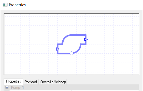
Pump components in TAS Systems allow the user to provide and control the flow rate of the fluid in the Plant Room.
Controllers
Controllers can be used with the pump component, and will control how much the pump will exert pressure on the fluid flowing through it.
The signal received by the pump dictates the proportion of the maximum pressure increase the pump will increase the pressure to.
Please note that this maximum pressure increase is not the value entered in the pumps’ Peak Pressure field. Instead the software will work the maximum pressure increase out by taking into account the Peak Pressure field of the pump, along with the design flow rates and design pressure drops of other components around the system.
Also, as pressure and flow rate are linked, controlling the pressure with a controller will also mean that the flow rate will vary. How the signal received by the pump affects the flow rate is shown using the equation below:
Commonly the sensor associated with the pump is placed onto the Collection and the controller is sensing the load of the Collection, turning the pump off when there’s no demand.
Properties
Name
This is the name of the component, it will be used in reports or error messages. You can rename components as you wish.
Description
The Description field allows the user to enter a description of the component. By default it is left blank.
Schedule
The Schedule field allows the user to apply a schedule to their component to detail the operational hours of the component.
If a schedule is applied by the user, then they should note that for all hours outside of the scheduled hours, the component will not operate.
In the case of the pump, this will mean that the pump will not provide any fluid flow. If all of your pumps in your system are scheduled to be off in the same hour then there will be no fluid flow in your system.
The default schedule option is always on, meaning that the component will operate 24/7.
Electrical Source
The Electrical Source field allows the user to decide the source of electricity for the Pumps.
The options given here will be any fuel source that is in the fuel source folder, so the user will be able to choose a non-electrical fuel source but this is not advised.
If the user chooses the “None” option, the user will receive a warning and the pump’s load will be discarded from the results.
Design Flow Rate
The Design Flow Rate field allows the user to set the design flow rate of the plant room fluid path the pump is on.
When the pump is on a loop with a collection with the Variable Flow Rate Option set to “No”, and the pump is not connected to a controller set up to vary the flow rate, then the design flow rate will be the flow rate of the fluid path.
If the Variable Flow Rate option is set to “Yes”, the pump is on the same circuit as a valve which is varying the flow, or the pump is connected to a controller set up to vary the flow then the design flow rate is the maximum flow rate of the fluid path.
There are two options available to set the design flow rate:
Value
Auto
Value
Upon choosing this option the user will enter the desired Design Flow Rate
Auto
Upon choosing this option the design flow rate will be sized upon the properties of components / collections with a Design Flow Delta T field, which are on the same circuit loop as the Pump.
If the component has “none” entered in the Design Flow Delta T field, it will be ignored for the sizing of the design flow rate by the pump. If a value is entered, TAS will size the design flow rate using the Design Flow Delta T field along with the peak load of the component.
The sizing is done such that the fluid is kept within the delta T temp limit when passing through the component and so that the demand of the component / collection is met.
Please note that for a collection it will just use the Design Flow Delta T field.
If a Design Flow Delta T is entered into 2 or more components / collections on the same circuit as the pump, TAS will use the component / collection which results in the larger design flow rate to size the design flow rate.
Overall Efficiency
The overall efficiency of the pump is its motor efficiency multiplied by the electrical efficiency.
Please note that this does not include any partload efficiency, which is set by the Partload field.
The user will need to enter the overall efficiency as a factor between zero and one.
Partload
Clicking on the Partload field will take you to the Partload Tab. From this tab, you will be able to edit the Partload profile of the component by using the graph or the table.
To see how to edit the Partload profiles, please watch the Profiles video in the TAS Systems User Guide.
Peak Pressure
The Peak Pressure of the pump is the upper limit on the amount of pressure the pump can generate.
The user should bear in mind that the peak pressure needs to satisfy the following equation, or otherwise they will receive a flow sizing error:
Control Type
This field allows the user to set the control type of the pump.
This option is only available when there is no controller attached to the pump. There are two options to choose from:
Variable Speed
Fixed Speed
Variable Speed
With this option the pressure generated at the Pump will match the sum of the pressure drops of the circuit, even if the peak pressure is larger.
Fixed Speed
The pressure generated at the pump will depend on the Variable Flow Option at the collection. If the Variable Flow Option is set to “No”, then the pressure generated at the pump will be equal to the sum of the pressure drops. If the Variable Flow Option is set to “Yes” then the Pressure generated at the Pump will vary between the Peak Pressure and the sum of all Pressure Drops on the circuit.
Tank
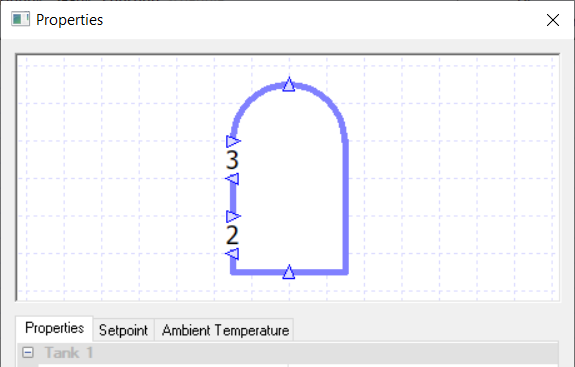
The Tank component allows for the storage of fluids in TAS Systems.
The tank has three fluid loops which connect to it.
The first loop, known as the Tank loop, models the fluid being stored in the tank. This loop enters the Tank component at the bottom port and exits the Tank component at the top port.
The other two loops, called Loop 2 and Loop 3, attach to the side of the tank and are heat exchanger loops which allow for heat transfer to the stored fluid.
When you click on the Tank component, the numbers 2 and 3 appear to denote which ports correspond to Loop 2 and which ports correspond to Loop 3.
Please note that it is not required to use both heat exchanger loops, but you do need to use at least one of them.
It is assumed that the tank is cylindrical.
No controllers may be used with this component.
Properties
Name
This is the name of the component, it will be used in reports or error messages. You can rename components as you wish.
Description
The Description field allows the user to enter a description of the component. By default it is left blank.
Insulation Conductivity
The user will need to enter the thermal conductivity of the tank’s insulation.
Insulation Thickness
In this field, the user enters the thickness of the tank’s insulation.
Design Pressure Drop (Tank)
This field allows the user to enter the design pressure drop of the fluid being stored in the tank; which is the fluid entering the tank from the bottom port and exiting from the top port.
The drop in pressure is caused by resistance to the flow and the value entered will affect the amount of energy used by the pump on this circuit loop.
If the “Not Used” option is selected for this field, the user will be asked to enter in a Capacity of the fluid loop through this component.
Design Pressure Drop (2)
This field allows the user to enter the design pressure drop for the fluid on Loop 2 when passing through the Tank component.
The drop in pressure is caused by resistance to the flow and the value entered will affect the amount of energy used by the pump on this circuit loop.
If the “Not Used” option is selected for this field, the user will be asked to enter in a Capacity of the fluid loop through this component.
Design Pressure Drop (3)
This field allows the user to enter the design pressure drop for the fluid on Loop 3 when passing through the Tank component.
The drop in pressure is caused by resistance to the flow and the value entered will affect the amount of energy used by the pump on this circuit loop.
If the “Not Used” option is selected for this field, the user will be asked to enter in a Capacity of the fluid loop through this component.
Volume
In this field the user enters the volume of the tank.
Height (Top to Bottom)
This field allows the user to enter the height of the tank.
Setpoint Method
With this field the user can decide their setpoint method. There are two choices:
Off – When set to Off, there is no setpoint for the temperature of the fluid in the tank. This means that heat will be exchanged by the heat exchanger loops for all operating hours.
On – Upon choosing this option, the user will be asked to enter a temperature as a setpoint. Once the fluid in the tank hits this temperature setpoint, the exchanger loops will bypass the tank to avoid any additional heating.
Heat Exchanger (2)
The Heat Exchanger (2) field allows the user to set the efficiency of the heat transfer between the tank and Loop 2.
The efficiency is set by the following formula:
Where \(\text{Loop2}_{\text{return}}\) is the temperature of the fluid leaving the tank on Loop 2, \(\text{Loop2}_{\text{supply}}\) is the temperature of the fluid entering the tank on Loop 2 and \(\text{Tank}_{\text{mean}}\) is the mean temperature of the tank for the hour which can be found by checking the temperature of the fluid leaving the tank at the top port.
Heat Exchanger (3)
The Heat Exchanger (3) field allows the user to set the efficiency of the heat transfer between the tank and Loop 3.
Please note that that the efficiency formula in the Heat Exchanger (2) field is used to calculate the efficiency here as well but with Loop 3 replacing all mentions of Loop 2.
Ambient Temperature Outside Tank
The user will input here the average temperature of the area where the tank is stored.
The user can go to the Ambient Temperature tab to set up a modifier with this field. They can also drag a zone, from the TSDData folder, onto the tank and Systems will use the zone’s temperature as the ambient temperature for each hour of the simulation.
Valve
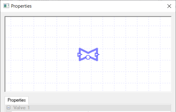
The Valve component for the plant room acts similarly to the Damper component for air side systems.
They are mainly used after splitting fluid paths, modulating the flow on each new path.
Please note that unlike the damper, the design flow rate must be entered manually here. So when splitting fluid paths you will need to check manually that the design flow rate on both sides, before and after the split, match.
Controllers
Controllers can be used with the valve, and they will control the capacity of the valve.
The signal the valve receives dictates the proportion of the maximum capacity that the valve will close to, where the maximum capacity is set by either the Design Flow Rate field or the Capacity field of the valve.
So for example, if the valve receives a signal of 1 from the controller, the valve will open up and allow fluid through it according to its maximum capacity.
If the valve receives a signal of zero from the controller, the valve will close completely and will not allow any fluid to pass through it.
It should be noted that as the capacity of the valve varies, the flow rate and pressure of the fluid around the system will also vary.
Properties
Name
This is the name of the component, it will be used in reports or error messages. You can rename components as you wish.
Description
The Description field allows the user to enter a description of the component. By default it is left blank.
Schedule
The Schedule field allows the user to apply a schedule to their component to detail the operational hours of the component.
If a schedule is applied by the user, then they should note that for all hours outside of the scheduled hours, the component will not operate.
In the case of the valve, this will mean that the valve will close and will not allow any fluid to flow through it. This will mean any other component on the same fluid path as the valve will not receive any fluid flow in this hour.
The default schedule option is always on, meaning that the component will operate 24/7.
Design Pressure Drop
This field allows the user to enter the pressure drop of the fluid when passing through the valve.
The drop in pressure is caused by resistance to the flow and the value entered will affect the amount of energy used by the pump on the loop.
If the “Not Used” option is selected for this field, the user will be asked to enter in a Capacity of the fluid loop through this valve.
Design Flow Rate
The Design Flow Rate field allows the user to set the design flow rate of the fluid path the valve is on.
When the valve is on a loop with a collection with the Variable Flow Option set to “No”, then the design flow rate will be the flow rate of the fluid path.
If the Variable Flow Rate option is set to “Yes” then the design flow rate is the maximum flow rate of the fluid path.
Please also note that the Design Flow Rate field for a pump and valve on the same fluid path must match. If the pump’s Design Flow Rate field is set to “auto” and a value is entered in the valve’s Design Flow Rate field, when the valve is on the same fluid path as the pump, then the pump will take the valve’s design flow rate.
There are two options to set the design flow rate:
Auto
Value
Auto
Upon choosing this option the design flow rate will be sized upon the properties of components / collections with a Design Flow Delta T field, which are on the same circuit loop as the Valve.
If the component has “none” entered in the Design Flow Delta T field, it will be ignored for the sizing of the design flow rate by the valve.
If a value is entered, TAS will size the design flow rate using the Design Flow Delta T field along with the peak load of the component. The sizing is done such that the fluid is kept within the delta T temp limit when passing through the component and so that the demand of the component / collection is met.
Please note that for a collection it will just use the Design Flow Delta T field. If a Design Flow Delta T is entered into 2 or more components / collections on the same circuit as the pump, TAS will use the component / collection which results in the larger design flow rate to size the design flow rate.
Value
Upon choosing this option the user will enter a value which will be used for the Design Flow Rate.
Design Flow Capacity Signal
The Design Flow Capacity Signal option only appears when a controller is attached to the component.
The design flow capacity signal allows the user to make the design flow rate of the damper correspond to a certain signal from the controller.
For instance if the Design Flow Capacity Signal field has the value x entered into it then when the controller’s signal reads x, the flow rate through the damper will be the design flow rate.
By design the factor is set to one by default and it is strongly recommended that it is kept that way.
Junction
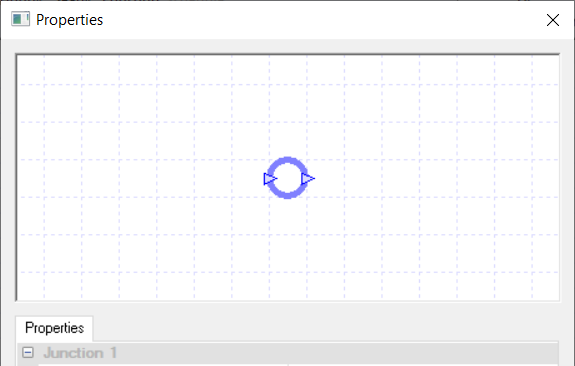
The Junction component has two uses.
The first use is to model where the fluid enters the system and where the fluid leaves the system. In these cases the junction will only have one duct connected to it and it will turn blue, to indicate it is an external junction.
The second use of a junction is to split or merge fluid paths. When being used to split fluid paths, a valve should be used in conjunction with the junction.
You cannot use controllers with junctions.
Properties
Name
This is the name of the component, it will be used in reports or error messages. You can rename components as you wish.
Description
The Description field allows the user to enter a description of the component. By default it is left blank.
Mains Pressure
This field allows the user to account for the fluid pressure their fluid is supplied at from the mains; due to this, this option only appears for external junctions.
If the user uses the “Off” option then the fluid is not pressurised when provided from the mains.
If the “On” option is chosen, the user needs to enter the pressure the fluid is supplied at from the mains.
When a pressure is modelled here, the user will not need to model a pump on the circuit loop, as the mains pressure will cause the fluid to flow. However, the user may want to model a valve on the circuit as a replacement to the pump, so they can turn off the flow when there is no demand.
Pipe Loss Components
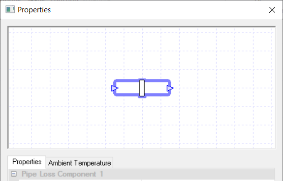
The Pipe Loss Component allows the user to model the heat loss / gain that the fluid will experience when travelling through pipes.
The user can model the pipes being placed in the ground or exposed to air.
Note that on simulation hours when the flow through this component is zero, the effect of the thermal mass of the fluid within the pipe is disregarded. In other words, it cannot be used for thermal storage, unlike the Tank component.
Please note that controllers cannot be used with this component.
Properties
Name
This is the name of the component, it will be used in reports or error messages. You can rename components as you wish.
Description
The Description field allows the user to enter a description of the component. By default it is left blank.
Design Pressure Drop
This field allows the user to enter the pressure drop of the fluid when it flows through the component.
The drop in pressure is caused by resistance to the flow and the value entered will affect the amount of energy used by the pump on the component’s circuit loop.
If the “Not Used” option is selected for this field, the user will be asked to enter in a Capacity of the fluid loop through this component.
Length
The user will input the length of the pipe in this field.
Pipe Inside Diameter
The user will input the inside diameter of the pipe.
Pipe Outside Diameter
The user should input the outside diameter of the pipe.
Pipe Conductivity
Please enter the thermal conductivity of the pipe, not including the insulation.
Insulation Thickness
Please enter here the thickness of your insulation.
Insulation Conductivity
Please enter here the thermal conductivity of the insulation.
Heat Exchange Type
This field allows the user to tell TAS if the pipe is in the ground, by setting the heat exchanger type to “With Ground”, or exposed to air, by setting the heat exchanger type to “With Air”.
Upon choosing the “With Ground” option, the user will have to enter the following information:
Ground Conductivity - This field requires the user to enter the thermal conductivity of the ground surrounding the pipe. If the soil type varies in the ground around the pipe then please take a weighted average for the ground conductivity.
Ground Heat Capacity - This field requires the user to enter the heat capacity of the ground surrounding the pipe. If the soil type varies in the ground around the pipe, then please take a weighted average for the specific heat capacity.
Ground Density - This field requires the user to enter the density of the ground that the pipe is placed into. If the soil type changes around the pipe then please take a weighted average for the density.
Undistributed Ground Temperature - This will be the temperature of the ground before any heat exchange. This can be entered as a value or set by using the “Set to Ground Water Temp” option. If using the latter option, it will be set using the Water Temperature option in the simulation dialog box.
If the user chooses the “With Air” option, they will be asked to enter the ambient air temperature of the air surrounding the pipe.
The user can use the Ambient Air Temperature tab to set up a modifier or yearly profile for this temperature. They can also drag a zone, from the TSDData folder, onto the pipe and Systems will use the zone’s temperature as the ambient temperature for each hour of the simulation.
Air Source Chiller
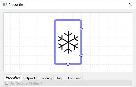
The Air Source Chiller component in TAS Systems allows users to model an air source chiller.
The two ports on the chiller represent where the fluid ducts connect to the chiller.
Controllers
You can use a controller with the chiller to control how the chiller behaves.
For a chiller, the controller controls it by informing it of the amount of power the chiller should use to cool down the fluid flowing through it.
The controller does this by sending a signal, between zero and one, to the chiller dictating the proportion of the chiller’s duty it should use to cool down the fluid.
So, for example, if the chiller received a signal of zero the chiller would not cool down the fluid flowing through it.
While if it received a signal of 1 the chiller will cool down the fluid flowing through it using the maximum amount of power allowed from the Duty field.
If no controller is used, the sensor used to determine the fluid’s temperature for the Setpoint field is assumed to be directly after the return port of the chiller.
Properties
Name
This is the name of the component, it will be used in reports or error messages. You can rename components as you wish.
Description
The Description field allows the user to enter a description of the component. By default it is left blank.
Schedule
The Schedule field allows the user to apply a schedule to their component to detail the operational hours of the component.
If a schedule is applied by the user, then they should note that for all hours outside of the scheduled hours, the component will not operate.
In the case of the air source chiller, this will mean that the fluid will flow through the chiller uncooled, even if there is a controller sending a non-zero signal to the chiller.
The default schedule option is always on, meaning that the component will operate 24/7.
Fuel Source
With this field the user can choose the fuel source of the air source chiller.
The options provided in the drop-down menu come from the fuel sources placed in the fuel source folder.
If no fuel sources have been placed in this folder, the only option available will be the “none” option.
If the “none” option is used, you will obtain a warning and the loads of the component will be discarded.
Fan Fuel Source
This option works in the same way as the Fuel Source option but allows the user to set the fuel source for the Air Source Chiller’s fan.
Design Pressure Drop
This field allows the user to enter the pressure drop of the fluid flowing through the component.
The drop in pressure is caused by resistance to the flow and the value entered will affect the amount of energy used by the pump on the chillers circuit.
If the “Not Used” option is selected for this field, the user will be asked to enter in a Capacity of the fluid loop through this component.
Setpoint
When a temperature is entered into the Setpoint field, the component will attempt to regulate the temperature of the fluid going through it to reach the setpoint.
In the case of the air source chiller, it will cool the fluid so it reaches the setpoint, but it will not be able to warm up the fluid to reach this setpoint. To heat the fluid you would need another component, for instance a boiler.
Please note that when a controller is used in conjunction with the chiller, the Setpoint field will disappear from the properties. This is done because the chiller is being controlled by a controller and will cool down the fluid when the controller sends a signal informing the chiller to do so.
When the Setpoint field is visible, modifiers can be added to the setpoint using the Setpoint tab.
Design Flow Delta T
The Design Flow Delta T field allows the user to size the flow rate of the circuit loop the component is on such that the fluid flowing through the component is kept within a certain temperature band.
The user can choose not to size the flow rate using this band, by choosing the “None” option.
If the user decides to use this option, by choosing the “Value” option, they will need to make sure that they have a pump on the same circuit loop as the component with the pump’s Design Flow Rate field set to “Sized”.
The value entered into the Design Flow Delta T field of the chiller affects the flow rate of the circuit loop in the following way. If the component has a setpoint of \(x\) and a Design Flow Delta T of \(y\), then the fluid will always be kept within the temperature range \(x-y\) to \(x+y\) when flowing through the component by ensuring the design flow rate of the circuit is sized high enough.
If multiple components / collections on the same circuit have a Design Flow Delta T value entered, TAS will take the results of the one which requires the highest design flow rate.
Please note that for components, the Design Flow Delta T will also size the flow rate so that the demand placed on the component is also met.
Efficiency
Upon clicking on the Efficiency field, you will be transferred over to the Efficiency tab where you can create a profile for the efficiency.
Normally the modifier chosen here would be a table modifier with a partload profile.
The efficiency input for a chiller should be the EER.
Duty
The duty of a component is the upper limit on the amount of power a component can provide.
If, in a certain hour, the power demand on the component is greater than the duty of the component, the component will not be able to meet this demand (For an air source chiller, it means it wouldn’t be able to cool the fluid to the setpoint, it would fall short).
In TAS Systems, the demand met by a component is reported for each hour in the results section.
Currently, there are 3 options for setting the duty:
Unlimited
Sized
Value
Unlimited
Unlimited means the component is always able to meet the demand. Please note that this option cannot be used when a controller is attached to the component.
Sized
Allows the user to size the duty on a design condition. The user will also be asked for a size fraction and a method to size on. With the method option, you get to choose from the following options:
Add load, all attached – TAS Systems will size the duty of the component on the demand from all attached collections in the circuit.
Add load, local – TAS systems will size the duty of the component on the demand from all collections on the same loop as the component.
Please note that to size the duty the user will need to have design conditions in their systems file.
Value
With this option the user will type in the duty of the component. In the duty tab, you will be able to choose these 3 options as well, but with the sized and value options you will be able to add a modifier.
Extra Fan Load
This field allows the user to model the load used by the fan in the chiller. The user will be taken to the modifier profile in the Fan Load tab, where you can edit the profile to reflect the partload profile of the fan in the chiller.
Water Source Chiller

The Water Source Chiller component in TAS Systems allows users to model water source chillers which transfer their load to another fluid loop.
Due to this the water source chiller requires connection to two circuit loops, one for providing the cooling to the collection and another for the rejected load.
The component has an arrow on it to indicate to what loop the load is being rejected. Also when you click on the component, the numbers 1 and 2 appear next to the ports to denote the loops.
The cooling collection loop should be connected to the ports on the side numbered 2 (the side of the arrow’s tail) while the heat rejection loop should be connected to the ports on the side numbered 1 (the side of the arrow’s point).
Controllers
You can use a controller with the chiller to control how the chiller behaves.
For a chiller, the controller controls it by informing it of the amount of power the chiller should use to cool down the fluid flowing through it.
The controller does this by sending a signal, between zero and one, to the chiller dictating the proportion of the chiller’s duty it should use to cool down the fluid.
So, for example, if the chiller received a signal of zero the chiller would not cool down the fluid flowing through it on the cooling loop. While if it received a signal of 1 the chiller will cool down the fluid flowing through it on the cooling loop using the maximum amount of power allowed from the Duty field.
If no controller is used, the sensor for determining the temperature of the fluid for the Setpoint field is assumed to be directly after the exit port on the cooling loop (side denoted with a 2).
Properties
Name
This is the name of the component, it will be used in reports or error messages. You can rename components as you wish.
Description
The Description field allows the user to enter a description of the component. By default it is left blank.
Schedule
The Schedule field allows the user to apply a schedule to their component to detail the operational hours of the component.
If a schedule is applied by the user, then they should note that for all hours outside of the scheduled hours, the component will not operate.
In the case of the water source chiller, this will mean that the fluid will flow through the cooling loop of the chiller uncooled and no heat would be rejected to the heat rejection loop, even if there is a controller sending a non-zero signal to the chiller.
The default schedule option is always on, meaning that the component will operate 24/7.
Fuel Source
With this field the user can choose the fuel source of the water source chiller.
The options provided in the drop-down menu come from the fuel sources placed in the fuel source folder, so the user will be able to choose a non-electrical fuel source but this is not advised.
If no fuel sources have been placed in this folder, the only option available will be the “none” option. If the “none” option is used, you will obtain a warning and the loads of the component will be discarded.
Ancillary Load Fuel Source
This option works in the same way as the Fuel Source option but allows the user to set the fuel source for the ancillary loads of the chiller.
Design Pressure Drop (1)
This field allows the user to enter the pressure drop of the fluid on the heat rejection loop when flowing through the component (This is the side marked with a 1 when you click on the component).
The drop in pressure is caused by resistance to the flow and the value entered will affect the amount of energy used by the pump on the heat rejection loop.
If the “Not Used” option is selected for this field, the user will be asked to enter in a Capacity of the fluid loop through this component.
Design Pressure Drop (2)
This field allows the user to enter the pressure drop of the fluid on the cooling loop when flowing through the component (This is the side marked with a 2 when you click on the component).
The drop in pressure is caused by resistance to the flow and the value entered will affect the amount of energy used by the pump on the cooling loop.
If the “Not Used” option is selected for this field, the user will be asked to enter in a Capacity of the fluid loop through this component.
Design Flow Delta T (1)
The Design Flow Delta T (1) field allows the user to size the flow rate of the heat rejection loop of the component such that the fluid flowing through the component is kept within a certain temperature band (Please note that this is the loop marked with a 1 when you click on the component).
The user can choose not to size the flow rate using this band, by choosing the “None” option.
If the user decides to use this option, by choosing the “Value” option, they will need to make sure that they have a pump on the same circuit loop as the component with the pump’s Design Flow Rate field set to “Sized”.
The value entered into the Design Flow Delta T field of the chiller affects the flow rate of the circuit loop in the following way. If the component has a setpoint of x and a Design Flow Delta T of y, then the fluid will always be kept within the temperature range \(x-y\) to \(x+y\) when flowing through the component by ensuring the design flow rate of the circuit is sized high enough.
If multiple components / collections on the same circuit have a Design Flow Delta T value entered, TAS will take the results of the one which requires the highest design flow rate.
Please note that for components, the Design Flow Delta T will also size the flow rate so that the demand placed on the component is also met.
Design Flow Delta T (2)
The Design Flow Delta T (2) field allows the user to size the flow rate of the cooling loop of the component such that the fluid flowing through the component is kept within a certain temperature band (Please note that this is the loop marked with a 2 when you click on the component).
Apart from this difference, it works in the same way as the Design Flow Delta T (1) field.
Setpoint
When a temperature is entered into the Setpoint field, the component will attempt to regulate the temperature of the fluid going through it to reach the setpoint.
In the case of the Water Source Chiller, it will cool the fluid so it reaches the setpoint, but it will not be able to warm up the fluid to reach this setpoint. To heat the fluid you would need another component, for instance a boiler.
Please note that when a controller is used in conjunction with the chiller, the Setpoint field will disappear from the properties. This is done because the chiller is being controlled by a controller and will cool down the fluid when the controller sends a signal informing the chiller to do so.
When the Setpoint field is visible, modifiers can be added to the setpoint using the Setpoint tab.
Efficiency
Upon clicking on the Efficiency field, you will be transferred over to the Efficiency tab where you can create a profile for the efficiency. Normally the modifier chosen here would be a table modifier with a partload profile.
The efficiency input for a chiller should be the EER.
Duty
The duty of a component is the upper limit on the amount of power a component can provide.
If, in a certain hour, the power demand on the component is greater than the duty of the component, the component will not be able to meet this demand (for a water source chiller, it means it wouldn’t be able to cool the fluid to the setpoint, it would fall short.).
In TAS Systems, the demand met by a component is reported for each hour in the results section.
Currently, there are 3 options for setting the duty:
Unlimited
Sized
Value
Unlimited
Unlimited means the component is always able to meet the demand. Please note that this option cannot be used when a controller is attached to the component.
Sized
Allows the user to size the duty on a design condition. The user will also be asked for a size fraction and a method to size on. With the method option, you get to choose from the following options:
Add load, all attached – TAS Systems will size the duty of the component on the demand from all attached collections in the circuit.
Add load, local – TAS systems will size the duty of the component on the demand from all collections on the same loop as the component.
Please note that to size the duty the user will need to have design conditions in their systems file.
Value
With this option the user will type in the duty of the component. In the duty tab, you will be able to choose these 3 options as well, but with the sized and value options you will be able to add a modifier.
Motor Efficiency
The Motor Efficiency field allows the user to set the chiller’s motor efficiency.
In effect, this property dictates what proportion of the heat created due to the consumption is transferred to the heat rejection loop.
The user enters in a percentage into this field and this percentage of the heat generated due to the consumption is transferred over to the heat rejection loop.
If the efficiency is less than 100%, some of the heat created due to the consumption will be emitted outside of the chiller rather than being transferred to the heat rejection loop.
For example, if the Motor Efficiency is 85%, this implies that 15% of the energy associated with the chiller consumption is expended outside the chiller, and 85% becomes heat within the chiller itself (and this heat is added to the heat rejection loop).
Free Cooling
With this field, the user can decide if they want the Water Source Chiller component to model a heat exchanger exchanging heat between the heat rejection and cooling loops situated before the water source chiller (akin to a water side economiser setup).
There are three options to choose from:
None – Selecting this option means that no heat exchanger will be modelled.
On/Off - The heat exchanger will only exchange heat between the heat rejection and cooling loops when the entire cooling demand can be met by the heat exchange. Otherwise, no heat will be exchanged and the chiller will solely meet the cooling demand.
Variable - The heat exchanger will exchange heat between the heat rejection and cooling loops when part of the cooling demand can be met by the heat exchange. The remaining demand will be met by the chiller.
Calculation Method
This option allows the user to set up how the heat exchanger efficiency will be calculated when the Chiller is in free cooling mode. The user has the following two options:
Efficiency
NTU Method
Efficiency
Upon choosing this option the user is asked to enter the efficiency of the heat transfer. The efficiency of the heat transfer is calculated by the following formula:
Where \(\text{Cooling}_\text{out}\) is the temperature of the fluid leaving the chiller on the Cooling Collection loop, \(\text{Cooling}_\text{in}\) is the temperature of the fluid entering the chiller on the Cooling Collection loop and \(\text{Heat}_\text{in}\) is the temperature of the fluid entering the chiller on the Heat Rejection loop.
Please note that in the efficiency Tab, you can add a modifier to the Efficiency.
NTU Method
The second calculation method is the NTU method. Upon choosing this method, the user will need to input: The heat transfer surface area, the heat transfer coefficient and the exchanger type. After entering these details, TAS will then work out the rate of heat transfer of the Exchanger.
Ancillary Load
This field allows the user to model the load used by any additional ancillary services associated with the chiller.
Any value entered here will be the associated load during any hour the chiller operates, so it is advised to make use of the modifiers available with this field.
Modifiers can be added to this field using the Ancillary Load tab. Examples of ancillary loads which might be associated with plantroom components include internal pumps and fans which are not accounted for in the consumption figure for the component.
Multi Chiller
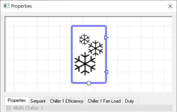
The Multi Chiller component allows the user to model multiple air source chillers using only one component.
Please note that any field beginning with “Chiller X …”, where X is a positive integer, is unique to the Xth air source chiller. The other fields (apart from: duty, sequence and multiplicity) are shared by all the chillers. So if the Multi Chiller is modelling 3 air source chillers, then each chiller will have the same setpoint while their fuel sources will be dependent on the field “Chiller X fuel source “.
Properties
As air source chillers have been discussed previously, only the new properties will be discussed.
Multiplicity
The number in the Multiplicity field represents how many chillers the Multi Chiller is representing.
Chiller X Percentage
This option allows the user to set the duty of the Xth chiller. The user will enter a percentage in this field which will set the chillers duty as this percentage of the total duty in the duty field.
Please note that the sum of all the “Chiller X Percentage” fields must add up to 100%. Not doing so will give you a warning and incorrect results.
Sequence
The Sequence field tells the component how the multiple chillers will be set up. The user has three options to choose from:
Parallel – The load is split up between the chillers. The load will be split evenly until one of the chillers reaches its duty.
Serial – The first chiller covers the load until it reaches its duty. At that point the second chiller would start to cover the load and so on.
Staged – With a staged setup only the first chiller runs at part load. As the first chiller normally has a bigger duty than the other chillers, once one of the other chillers can run at full load the load will transition to that chiller.
Absorption Chiller
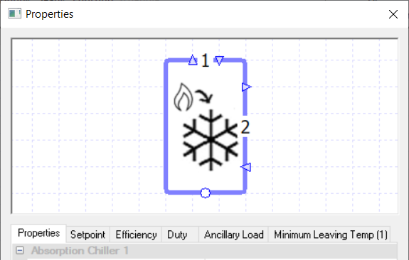
The absorption chiller is an air source chiller that uses a heat source to provide the energy to drive the cooling system.
Please note that as the heat source is providing the energy to the chiller, the demand on the heat source will match the consumption of the chiller.
If the heat source cannot meet this demand then the absorption chiller will not have enough energy to meet the cooling demand.
The Absorption Chiller component has two loops, which are denoted 1 and 2 when the component is selected. The loop denoted 1, called Loop 1, should be the loop containing the heat source. The loop denoted 2, called Loop 2, should be the loop containing the Cooling collection.
Controllers
You can use a controller with the chiller to control how the chiller behaves.
For an absorption chiller, the controller controls it by informing it of the amount of power the absorption chiller should use to cool down the fluid flowing through it on Loop 2 (the cooling loop).
The controller does this by sending a signal, between zero and one, to the chiller dictating the proportion of the chiller’s duty it should use to cool down the fluid.
So, for example, if the chiller received a signal of zero the chiller would not cool down the fluid flowing through it. While if it received a signal of 1 the chiller will cool down the fluid flowing through it using the maximum amount of power allowed from the Duty field.
If no controller is used, the sensor used to determine the fluid’s temperature for the Setpoint field is assumed to be directly after Loop 2’s return port.
Properties
Name
This is the name of the component, it will be used in reports or error messages. You can rename components as you wish.
Description
The Description field allows the user to enter a description of the component. By default it is left blank.
Design Pressure Drop (1)
This field allows the user to enter the pressure drop of the fluid on Loop 1 (The loop containing the heat source providing the energy for the absorption chiller) when passing through the absorption chiller.
The drop in pressure is caused by resistance to the flow and the value entered will affect the amount of energy used by the pump on the left loop’s circuit.
If the “Not Used” option is selected for this field, the user will be asked to enter in a Capacity of the fluid loop through this component.
Design Pressure Drop (2)
This field allows the user to enter the pressure drop of the fluid on Loop 2 (The loop containing the Cooling Collection on the side of the absorption chiller) when passing through the absorption chiller.
The drop in pressure is caused by resistance to the flow and the value entered will affect the amount of energy used by the pump on the right loop’s circuit.
If the “Not Used” option is selected for this field, the user will be asked to enter in a Capacity of the fluid loop through this component.
Setpoint
When a temperature is entered into the Setpoint field, the component will attempt to regulate the temperature of the fluid going through it to reach the setpoint.
In the case of the absorption chiller, it will cool the fluid on Loop 2 (the cooling loop) so it reaches the setpoint, but it will not be able to warm up the fluid to reach this setpoint. To heat the fluid you would need another component, for instance a boiler.
Please note that when a controller is used in conjunction with the chiller, the Setpoint field will disappear from the properties. This is done because the chiller is being controlled by a controller and will cool down the fluid when the controller sends a signal informing the chiller to do so.
When the Setpoint field is visible, modifiers can be added to the setpoint using the Setpoint tab.
Efficiency
Upon clicking on the Efficiency field, you will be transferred over to the Efficiency tab where you can create a profile for the efficiency. Normally the modifier chosen here would be a table modifier with a partload profile.
The efficiency input for a chiller should be the EER.
Duty
The duty of a component is the upper limit on the amount of power a component can provide.
If, in a certain hour, the power demand on the component is greater than the duty of the component, the component will not be able to meet this demand (for an absorption chiller, it means it wouldn’t be able to cool the fluid to the setpoint, it would fall short).
In TAS Systems, the demand met by a component is reported for each hour in the results section.
Currently, there are 3 options for setting the duty:
Unlimited
Sized
Value
Unlimited
Unlimited means the component is always able to meet the demand. Please note that this option cannot be used when a controller is attached to the component.
Sized
Allows the user to size the duty on a design condition. The user will also be asked for a size fraction and a method to size on. With the method option, you get to choose from the following options:
Add load, all attached – TAS Systems will size the duty of the component on the demand from all attached collections in the circuit.
Add load, local – TAS systems will size the duty of the component on the demand from all collections on the same loop as the component.
Please note that to size the duty the user will need to have design conditions in their systems file.
Value
With this option the user will type in the duty of the component. In the duty tab, you will be able to choose these 3 options as well, but with the sized and value options you will be able to add a modifier.
Minimum Leaving Temperature (1)
This field sets a minimum leaving temperature for the fluid flowing through the absorption chiller on Loop 1 (i.e. the loop containing the heat source).
Please note that setting this minimum return temperature too high can lead to the absorption chiller not receiving enough heat to meet the cooling demand.
Modifiers can be added to this field by selecting the Minimum Leaving Temperature (1) tab.
Ancillary Load Fuel Source
With this field the user can choose the fuel source of the ancillary loads associated with the absorption chiller.
The options provided in the drop-down menu come from the fuel sources placed in the fuel source folder.
If no fuel sources have been placed in this folder, the only option available will be the “none” option. If the “none” option is used, you will obtain a warning and any entered ancillary loads of the component will be discarded.
Ancillary Load
This field allows the user to model the load used by any additional ancillary services associated with the chiller.
Any value entered here will be the associated load during any hour the chiller operates, so it is advised to make use of the modifiers available with this field.
Examples of ancillary loads which might be associated with plantroom components include internal pumps and fans which are not accounted for in the consumption figure for the component.
Modifiers can be added to this field using the Ancillary Load tab.
Air Source Direct Absorption Chiller
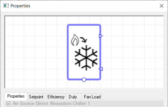
The Air Source Direct Absorption Chiller component acts like an absorption chiller, but does not require a separate loop containing the absorption chiller’s heat source to be modelled. Instead, the Efficiency field of the chiller would account for the absorption chiller creating the heat and then using it to power the cooling.
The two ports on the chiller represent where the fluid ducts connect to the chiller.
Controllers
You can use a controller with the chiller to control how the chiller behaves. For a chiller, the controller controls it by informing it of the amount of power the chiller should use to cool down the fluid flowing through it.
The controller does this by sending a signal, between zero and one, to the chiller dictating the proportion of the chiller’s duty it should use to cool down the fluid.
So, for example, if the chiller received a signal of zero the chiller would not cool down the fluid flowing through it. While if it received a signal of 1 the chiller will cool down the fluid flowing through it using the maximum amount of power allowed from the Duty field.
If no controller is used, the sensor used to determine the fluid’s temperature for the Setpoint field is assumed to be directly after the return port of the chiller.
Properties
Name
This is the name of the component, it will be used in reports or error messages. You can rename components as you wish.
Description
The Description field allows the user to enter a description of the component. By default it is left blank.
Schedule
The Schedule field allows the user to apply a schedule to their component to detail the operational hours of the component.
If a schedule is applied by the user, then they should note that for all hours outside of the scheduled hours, the component will not operate.
In the case of the air source direct absorption chiller, this will mean that the fluid will flow through the chiller uncooled, even if there is a controller sending a non-zero signal to the chiller.
The default schedule option is always on, meaning that the component will operate 24/7.
Fuel Source
With this field the user can choose the fuel source of the air source direct absorption chiller.
The options provided in the drop-down menu come from the fuel sources placed in the fuel source folder. If no fuel sources have been placed in this folder, the only option available will be the “none” option.
If the “none” option is used, you will obtain a warning and the loads of the component will be discarded.
Fan Fuel Source
This option works in the same way as the Fuel Source option but allows the user to set the fuel source for the air source direct absorption chiller’s fan.
Design Pressure Drop
This field allows the user to enter the pressure drop of the fluid flowing through the component.
The drop in pressure is caused by resistance to the flow and the value entered will affect the amount of energy used by the pump on the chillers circuit.
If the “Not Used” option is selected for this field, the user will be asked to enter in a Capacity of the fluid loop through this component.
Setpoint
When a temperature is entered into the Setpoint field, the component will attempt to regulate the temperature of the fluid going through it to reach the setpoint.
In the case of the air source direct absorption chiller, it will cool the fluid so it reaches the setpoint, but it will not be able to warm up the fluid to reach this setpoint. To heat the fluid you would need another component, for instance a boiler.
Please note that when a controller is used in conjunction with the chiller, the Setpoint field will disappear from the properties. This is done because the chiller is being controlled by a controller and will cool down the fluid when the controller sends a signal informing the chiller to do so.
When the Setpoint field is visible, modifiers can be added to the setpoint using the Setpoint tab.
Design Flow Delta T
The Design Flow Delta T field allows the user to size the flow rate of the circuit loop the component is on such that the fluid flowing through the component is kept within a certain temperature band.
The user can choose not to size the flow rate using this band, by choosing the “None” option. If the user decides to use this option, by choosing the “Value” option, they will need to make sure that they have a pump on the same circuit loop as the component with the pump’s Design Flow Rate field set to “Sized”.
The value entered into the Design Flow Delta T field of the chiller affects the flow rate of the circuit loop in the following way. If the component has a setpoint of \(x\) and a Design Flow Delta T of \(y\), then the fluid will always be kept within the temperature range \(x-y\) to \(x+y\) when flowing through the component by ensuring the design flow rate of the circuit is sized high enough.
If multiple components / collections on the same circuit have a Design Flow Delta T value entered, TAS will take the results of the one which requires the highest design flow rate.
Please note that for components, the Design Flow Delta T will also size the flow rate so that the demand placed on the component is also met.
Efficiency
Upon clicking on the Efficiency field, you will be transferred over to the Efficiency tab where you can create a profile for the efficiency.
Normally the modifier chosen here would be a table modifier with a partload profile.
Please note that for the air source direct absorption chiller, the Efficiency of the chiller would account for the absorption chiller creating the heat and then using it to power the cooling.
Duty
The duty of a component is the upper limit on the amount of power a component can provide.
If, in a certain hour, the power demand on the component is greater than the duty of the component, the component will not be able to meet this demand (for an air source direct absorption chiller, it means it wouldn’t be able to cool the fluid to the setpoint, it would fall short).
In TAS Systems, the demand met by a component is reported for each hour in the results section.
Currently, there are 3 options for setting the duty:
Unlimited
Sized
Value
Unlimited
Unlimited means the component is always able to meet the demand. Please note that this option cannot be used when a controller is attached to the component.
Sized
Allows the user to size the duty on a design condition. The user will also be asked for a size fraction and a method to size on. With the method option, you get to choose from the following options:
Add load, all attached – TAS Systems will size the duty of the component on the demand from all attached collections in the circuit.
Add load, local – TAS systems will size the duty of the component on the demand from all collections on the same loop as the component.
Please note that to size the duty the user will need to have design conditions in their systems file.
Value
With this option the user will type in the duty of the component. In the duty tab, you will be able to choose these 3 options as well, but with the sized and value options you will be able to add a modifier.
Extra Fan Load
This field allows the user to model the load used by the fan in the chiller.
The user will be taken to the modifier profile in the Fan Load tab, where you can edit the profile to reflect the partload profile of the fan in the chiller.
Water – Source Absorption Chiller
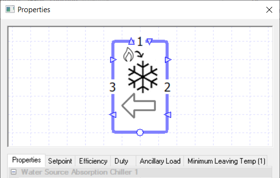
The water source absorption chiller acts in much the same way as the absorption chiller but instead of rejecting the heat to the air, it rejects it to a heat rejection fluid loop.
Due to the additional heat rejection loop, the Water Source Absorption Chiller component has three loops, which are denoted 1, 2 and 3 when the component is selected.
The loop denoted 1, called Loop 1, should be the loop containing the heat source. The loop denoted 2, called Loop 2, should be the loop containing the Cooling collection, while the loop denoted 3, called Loop 3, should be the heat rejection loop.
Controllers
You can use a controller with the chiller to control how the chiller behaves.
For a water source absorption chiller, the controller controls it by informing it of the amount of power the absorption chiller should use to cool down the fluid flowing through it on Loop 2 (the cooling loop).
The controller does this by sending a signal, between zero and one, to the chiller dictating the proportion of the chiller’s duty it should use to cool down the fluid.
So, for example, if the chiller received a signal of zero the chiller would not cool down the fluid flowing through it. While if it received a signal of 1 the chiller will cool down the fluid flowing through it using the maximum amount of power allowed from the Duty field.
If no controller is used, the sensor used to determine the fluid’s temperature for the Setpoint field is assumed to be directly after Loop 2’s return port.
Properties
Name
This is the name of the component, it will be used in reports or error messages. You can rename components as you wish.
Description
The Description field allows the user to enter a description of the component. By default it is left blank.
Design Pressure Drop (1)
This field allows the user to enter the pressure drop of the fluid on Loop 1 (the loop containing the heat source providing the energy for the water source absorption chiller) when passing through the water source absorption chiller.
The drop in pressure is caused by resistance to the flow and the value entered will affect the amount of energy used by the pump on the left loop’s circuit.
If the “Not Used” option is selected for this field, the user will be asked to enter in a Capacity of the fluid loop through this component.
Design Pressure Drop (2)
This field allows the user to enter the pressure drop of the fluid on Loop 2 (the loop containing the Cooling Collection on the side of the water source absorption chiller) when passing through the water source absorption chiller.
The drop in pressure is caused by resistance to the flow and the value entered will affect the amount of energy used by the pump on the left loop’s circuit.
If the “Not Used” option is selected for this field, the user will be asked to enter in a Capacity of the fluid loop through this component.
Design Pressure Drop (3)
This field allows the user to enter the pressure drop of the fluid on Loop 3 (the heat rejection loop of the water source absorption chiller) when passing through the water source absorption chiller.
The drop in pressure is caused by resistance to the flow and the value entered will affect the amount of energy used by the pump on the left loop’s circuit.
If the “Not Used” option is selected for this field, the user will be asked to enter in a Capacity of the fluid loop through this component.
Setpoint
When a temperature is entered into the Setpoint field, the component will attempt to regulate the temperature of the fluid going through it to reach the setpoint.
In the case of the water source absorption chiller, it will cool the fluid on Loop 2 (the cooling loop) so it reaches the setpoint, but it will not be able to warm up the fluid to reach this setpoint. To heat the fluid you would need another component, for instance a boiler.
Please note that when a controller is used in conjunction with the chiller, the Setpoint field will disappear from the properties. This is done because the chiller is being controlled by a controller and will cool down the fluid when the controller sends a signal informing the chiller to do so.
When the Setpoint field is visible, modifiers can be added to the setpoint using the Setpoint tab.
Efficiency
Upon clicking on the Efficiency field, you will be transferred over to the Efficiency tab where you can create a profile for the efficiency. Normally the modifier chosen here would be a table modifier with a partload profile.
The efficiency input for a chiller should be the EER.
Duty
The duty of a component is the upper limit on the amount of power a component can provide.
If, in a certain hour, the power demand on the component is greater than the duty of the component, the component will not be able to meet this demand (for a water source absorption chiller, it means it wouldn’t be able to cool the fluid to the setpoint, it would fall short).
In TAS Systems, the demand met by a component is reported for each hour in the results section.
Currently, there are 3 options for setting the duty:
Unlimited
Sized
Value
Unlimited
Unlimited means the component is always able to meet the demand. Please note that this option cannot be used when a controller is attached to the component.
Sized
Allows the user to size the duty on a design condition. The user will also be asked for a size fraction and a method to size on. With the method option, you get to choose from the following options:
Add load, all attached – TAS Systems will size the duty of the component on the demand from all attached collections in the circuit.
Add load, local – TAS systems will size the duty of the component on the demand from all collections on the same loop as the component.
Please note that to size the duty the user will need to have design conditions in their systems file.
Value
With this option the user will type in the duty of the component. In the duty tab, you will be able to choose these 3 options as well, but with the sized and value options you will be able to add a modifier.
Minimum Leaving Temperature (1)
This field sets a minimum leaving temperature for the fluid flowing through the water source absorption chiller on Loop 1 (i.e. the loop containing the heat source).
Please note that setting this minimum return temperature too high can lead to the absorption chiller not receiving enough heat to meet the cooling demand.
Modifiers can be added to this field by selecting the Minimum Leaving Temperature (1) tab.
Ancillary Load Fuel Source
This field allows the user to model the load used by any additional ancillary services associated with the chiller.
Any value entered here will be the associated load during any hour the chiller operates, so it is advised to make use of the modifiers available with this field.
Examples of ancillary loads which might be associated with plantroom components include internal pumps and fans which are not accounted for in the consumption figure for the component.
Modifiers can be added to this field using the Ancillary Load tab.
Water Source Direct Absorption Chiller
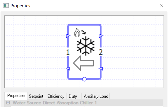
The water source direct absorption chiller acts in much the same way as the air source direct absorption chiller but instead of rejecting the heat to the air; it rejects it to a heat rejection fluid loop.
Due to the additional heat rejection loop, the Water Source Direct Absorption Chiller component has two loops, which are denoted 1 and 2 when the component is selected.
The loop denoted 1, called Loop 1, is the heat rejection loop. The loop denoted 2, called Loop 2, should be the loop containing the Cooling collection.
Controllers
You can use a controller with the chiller to control how the chiller behaves.
For a chiller, the controller controls it by informing it of the amount of power the chiller should use to cool down the fluid flowing through it.
The controller does this by sending a signal, between zero and one, to the chiller dictating the proportion of the chiller’s duty it should use to cool down the fluid.
So, for example, if the chiller received a signal of zero the chiller would not cool down the fluid flowing through it on the cooling loop. While if it received a signal of 1 the chiller will cool down the fluid flowing through it on the cooling loop using the maximum amount of power allowed from the Duty field.
If no controller is used, the sensor for determining the temperature of the fluid for the Setpoint field is assumed to be directly after the exit port on the cooling loop (side denoted with a 2).
Properties
Name
This is the name of the component, it will be used in reports or error messages. You can rename components as you wish.
Description
The Description field allows the user to enter a description of the component. By default it is left blank.
Schedule
The Schedule field allows the user to apply a schedule to their component to detail the operational hours of the component.
If a schedule is applied by the user, then they should note that for all hours outside of the scheduled hours, the component will not operate.
In the case of the water source direct absorption chiller, this will mean that the fluid will flow through the cooling loop of the chiller uncooled and no heat would be rejected to the heat rejection loop, even if there is a controller sending a non-zero signal to the chiller.
The default schedule option is always on, meaning that the component will operate 24/7.
Fuel Source
With this field the user can choose the fuel source of the water source direct absorption chiller.
The options provided in the drop down menu come from the fuel sources placed in the fuel source folder. If no fuel sources have been placed in this folder, the only option available will be the “none” option.
If the “none” option is used, you will obtain a warning and the loads of the component will be discarded.
Ancillary Load Fuel Source
This option works in the same way as the Fuel Source option but allows the user to set the fuel source for the ancillary loads of the chiller.
Design Pressure Drop (1)
This field allows the user to enter the pressure drop of the fluid on the heat rejection loop when flowing through the component (This is the side marked with a 1 when you click on the component).
The drop in pressure is caused by resistance to the flow and the value entered will affect the amount of energy used by the pump on the heat rejection loop.
If the “Not Used” option is selected for this field, the user will be asked to enter in a Capacity of the fluid loop through this component.
Design Pressure Drop (2)
This field allows the user to enter the pressure drop of the fluid on the cooling loop when flowing through the component (This is the side marked with a 2 when you click on the component).
The drop in pressure is caused by resistance to the flow and the value entered will affect the amount of energy used by the pump on the cooling loop.
If the “Not Used” option is selected for this field, the user will be asked to enter in a Capacity of the fluid loop through this component.
Design Flow Delta T (1)
The Design Flow Delta T (1) field allows the user to size the flow rate of the heat rejection loop of the component such that the fluid flowing through the component is kept within a certain temperature band (Please note that this is the loop marked with a 1 when you click on the component).
The user can choose not to size the flow rate using this band, by choosing the “None” option. If the user decides to use this option, by choosing the “Value” option, they will need to make sure that they have a pump on the same circuit loop as the component with the pump’s Design Flow Rate field set to “Sized”.
The value entered into the Design Flow Delta T field of the chiller affects the flow rate of the circuit loop in the following way. If the component has a setpoint of \(x\) and a Design Flow Delta T of \(y\), then the fluid will always be kept within the temperature range \(x-y\) to \(x+y\) when flowing through the component by ensuring the design flow rate of the circuit is sized high enough.
If multiple components / collections on the same circuit have a Design Flow Delta T value entered, TAS will take the results of the one which requires the highest design flow rate.
Please note that for components, the Design Flow Delta T will also size the flow rate so that the demand placed on the component is also met.
Design Flow Delta T (2)
The Design Flow Delta T (2) field allows the user to size the flow rate of the cooling loop of the component such that the fluid flowing through the component is kept within a certain temperature band (Please note that this is the loop marked with a 2 when you click on the component).
Apart from this difference, it works in the same way as the Design Flow Delta T (1) field.
Setpoint
When a temperature is entered into the Setpoint field, the component will attempt to regulate the temperature of the fluid going through it to reach the setpoint.
In the case of the water source direct absorption chiller, it will cool the fluid so it reaches the setpoint, but it will not be able to warm up the fluid to reach this setpoint. To heat the fluid you would need another component, for instance a boiler.
Please note that when a controller is used in conjunction with the chiller, the Setpoint field will disappear from the properties. This is done because the chiller is being controlled by a controller and will cool down the fluid when the controller sends a signal informing the chiller to do so.
When the Setpoint field is visible, modifiers can be added to the setpoint using the Setpoint tab.
Efficiency
Upon clicking on the Efficiency field, you will be transferred over to the Efficiency tab where you can create a profile for the efficiency.
Normally the modifier chosen here would be a table modifier with a partload profile.
Please note that for the water source direct absorption chiller, the Efficiency of the chiller would account for the absorption chiller creating the heat and then using it to power the cooling.
Duty
The duty of a component is the upper limit on the amount of power a component can provide.
If, in a certain hour, the power demand on the component is greater than the duty of the component, the component will not be able to meet this demand (for a water source direct absorption chiller, it means it wouldn’t be able to cool the fluid to the setpoint, it would fall short).
In TAS Systems, the demand met by a component is reported for each hour in the results section.
Currently, there are 3 options for setting the duty:
Unlimited
Sized
Value
Unlimited
Unlimited means the component is always able to meet the demand. Please note that this option cannot be used when a controller is attached to the component.
Sized
Allows the user to size the duty on a design condition. The user will also be asked for a size fraction and a method to size on. With the method option, you get to choose from the following options:
Add load, all attached – TAS Systems will size the duty of the component on the demand from all attached collections in the circuit.
Add load, local – TAS systems will size the duty of the component on the demand from all collections on the same loop as the component.
Please note that to size the duty the user will need to have design conditions in their systems file.
Value
With this option the user will type in the duty of the component. In the duty tab, you will be able to choose these 3 options as well, but with the sized and value options you will be able to add a modifier.
Free Cooling
With this field, the user can decide if they want the Water Source Direct Absorption Chiller component to model a heat exchanger exchanging heat between the heat rejection and cooling loops situated before the water source direct absorption chiller (akin to a water side economiser setup).
There are three options to choose from:
None – Selecting this option means that no heat exchanger will be modelled.
On/Off – The heat exchanger will only exchange heat between the heat rejection and cooling loops when the entire cooling demand can be met by the heat exchange. Otherwise, no heat will be exchanged and the chiller will solely meet the cooling demand.
Variable - The heat exchanger will exchange heat between the heat rejection and cooling loops when part of the cooling demand can be met by the heat exchange. The remaining demand will be met by the chiller.
Calculation Method
This option allows the user to set up how the heat exchanger efficiency will be calculated when the Chiller is in free cooling mode. The user has the following two options:
Efficiency
NTU Method
Efficiency
Upon choosing this option the user is asked to enter the efficiency of the heat transfer. The efficiency of the heat transfer is calculated by the following formula:
Where \(\text{Cooling}_\text{out}\) is the temperature of the fluid leaving the chiller on the Cooling Collection loop, \(\text{Cooling}_\text{in}\) is the temperature of the fluid entering the chiller on the Cooling Collection loop and \(\text{Heat}_\text{in}\) is the temperature of the fluid entering the chiller on the Heat Rejection loop.
Please note that in the efficiency Tab, you can add a modifier to the Efficiency.
NTU Method
The second calculation method is the NTU method. Upon choosing this method, the user will need to input: The heat transfer surface area, the heat transfer coefficient and the exchanger type. After entering these details, TAS will then work out the rate of heat transfer of the Exchanger.
Ancillary Load
This field allows the user to model the load used by any additional ancillary services associated with the chiller.
Any value entered here will be the associated load during any hour the chiller operates, so it is advised to make use of the modifiers available with this field.
Examples of ancillary loads which might be associated with plantroom components include internal pumps and fans which are not accounted for in the consumption figure for the component.
Modifiers can be added to this field using the Ancillary Load tab.
Ice Storage Chiller
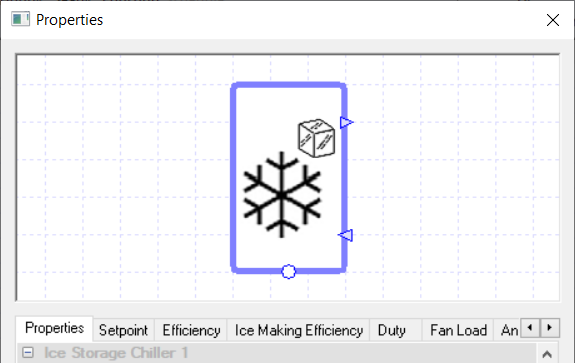
The ice storage chiller is an air source chiller but with the added ability to store excess cooling capacity as ice.
Controllers
You can use a controller with the chiller to control how the chiller behaves.
For a chiller, the controller controls it by informing it of the amount of power the chiller should use to cool down the fluid flowing through it.
The controller does this by sending a signal, between zero and one, to the chiller dictating the proportion of the chiller’s duty it should use to cool down the fluid.
So, for example, if the chiller received a signal of zero the chiller would not cool down the fluid flowing through it. While if it received a signal of 1 the chiller will cool down the fluid flowing through it using the maximum amount of power allowed from the Duty field.
If no controller is used, the sensor used to determine the fluid’s temperature for the Setpoint field is assumed to be directly after the return port of the chiller.
Properties
Name
This is the name of the component, it will be used in reports or error messages. You can rename components as you wish.
Description
The Description field allows the user to enter a description of the component. By default it is left blank.
Schedule
The Schedule field allows the user to apply a schedule to their component to detail the operational hours of the component.
If a schedule is applied by the user, then they should note that for all hours outside of the scheduled hours, the component will not operate.
In the case of the ice storage chiller, this will mean that the fluid will flow through the chiller uncooled, even if there is ice in the chiller.
The default schedule option is always on, meaning that the component will operate 24/7.
Fuel Source
With this field the user can choose the fuel source of the ice storage chiller.
The options provided in the drop-down menu come from the fuel sources placed in the fuel source folder. If no fuel sources have been placed in this folder, the only option available will be the “none” option.
If the “none” option is used, you will obtain a warning and the loads of the component will be discarded.
Fan Fuel Source
This option works in the same way as the Fuel Source option but allows the user to set the fuel source for the ice storage chiller’s fan.
Ancillary Load Fuel Source
This option works in the same way as the Fuel Source option but allows the user to set the fuel source for the ancillary loads of the chiller.
Design Pressure Drop
This field allows the user to enter the pressure drop of the fluid through the component.
The drop in pressure is caused by resistance to the flow and the value entered will affect the amount of energy used by the pump on the chillers circuit.
If the “Not Used” option is selected for this field, the user will be asked to enter in a Capacity of the fluid loop through this component.
Design Flow Delta T
The Design Flow Delta T field allows the user to size the flow rate of the circuit loop the component is on such that the fluid flowing through the component is kept within a certain temperature band.
The user can choose not to size the flow rate using this band, by choosing the “None” option. If the user decides to use this option, by choosing the “Value” option, they will need to make sure that they have a pump on the same circuit loop as the component with the pump’s Design Flow Rate field set to “Sized”.
The value entered into the Design Flow Delta T field of the chiller affects the flow rate of the circuit loop in the following way. If the component has a setpoint of \(x\) and a Design Flow Delta T of \(y\), then the fluid will always be kept within the temperature range \(x-y\) to \(x+y\) when flowing through the component by ensuring the design flow rate of the circuit is sized high enough.
If multiple components / collections on the same circuit have a Design Flow Delta T value entered, TAS will take the results of the one which requires the highest design flow rate.
Please note that for components, the Design Flow Delta T will also size the flow rate so that the demand placed on the component is also met.
Setpoint
When a temperature is entered into the Setpoint field, the component will attempt to regulate the temperature of the fluid going through it to reach the setpoint.
In the case of the ice storage chiller, it will cool the fluid so it reaches the setpoint, but it will not be able to warm up the fluid to reach this setpoint. To heat the fluid you would need another component, for instance a boiler.
Please note that when a controller is used in conjunction with the chiller, the Setpoint field will disappear from the properties. This is done because the chiller is being controlled by a controller and will cool down the fluid when the controller sends a signal informing the chiller to do so.
When the Setpoint field is visible, modifiers can be added to the setpoint using the Setpoint tab.
Efficiency
Upon clicking on the Efficiency field, you will be transferred over to the Efficiency tab where you can create a profile for the efficiency of the chiller.
Normally the modifier chosen here would be a table modifier with a partload profile.
The efficiency input for a chiller should be the EER.
Ice Making Efficiency
Like the Efficiency field, the Ice Making Efficiency field uses a modifier to create a Partload profile. The efficiency entered here is the efficiency of the ice storage chiller when making ice.
Duty
The duty of a component is the upper limit on the amount of power a component can provide.
If, in a certain hour, the power demand on the component is greater than the duty of the component, the component will not be able to meet this demand (for an ice storage chiller, it means that the cooling by duty will not be able to cover the demand. If any ice is being stored, the ice will be used to attempt to meet the demand).
In TAS Systems, the demand met by a component is reported for each hour in the results section.
Currently, there are 3 options for setting the duty:
Unlimited
Sized
Value
Unlimited
Unlimited means the component is always able to meet the demand. Please note that this option cannot be used when a controller is attached to the component.
Sized
Allows the user to size the duty on a design condition. The user will also be asked for a size fraction and a method to size on. With the method option, you get to choose from the following options:
Add load, all attached – TAS Systems will size the duty of the component on the demand from all attached collections in the circuit.
Add load, local – TAS systems will size the duty of the component on the demand from all collections on the same loop as the component.
Please note that to size the duty the user will need to have design conditions in their systems file.
Value
With this option the user will type in the duty of the component. In the duty tab, you will be able to choose these 3 options as well, but with the sized and value options you will be able to add a modifier.
Note that the “Unlimited” option which normally appears for component duty is not available for this property.
Ice Capacity
The Ice Capacity field allows the user to input the maximum amount of ice the ice storage chiller can store.
The user can determine how to set the capacity of the chiller from the following two options:
Sized – Allows the user to size the ice storage chiller during the simulation. An Hours at Full Load field will appear, allowing the user to enter how many hours of the chiller running at full load would it take to fully replenish the ice.
Value – With this option the user would type in the ice capacity into the software.
Initial Ice Reserve
The Initial Ice Reserve field allows the user to set the amount of stored ice the ice storage chiller has at the start of the simulation.
The user should enter the amount of ice stored as a percentage of the ice capacity.
Ice Melt Chiller Fraction
This field allows the user to enter in a minimum demand always met by the chiller’s duty, even when the chiller is set to prioritise cooling with ice.
This minimum demand is entered as a fraction of the duty, where zero would denote there is no minimum demand always met by the duty of the chiller.
Schedule: Cooling with Ice
This field allows the user to set a schedule dictating the hours where the chiller will prioritise cooling with Ice.
Taking into account the Ice Melt Chiller Fraction, the priority for cooling in these hours will be:
Outside of these hours, or in hours where the Cooling with Ice schedule clashes with the Making Ice schedule, the priority will be:
Schedule: Making Ice
This field allows the user to set a schedule on when the chiller will make ice.
Please be aware that outside of scheduled hours, the chiller will not cool using this functionality. Also if all of the chiller’s duty is used up meeting the Cooling demand, then the chiller will not be able to create ice.
Extra Fan Load
This field allows the user to model the load used by the fan in the chiller.
The user will be taken to the modifier profile in the Fan Load tab, where you can edit the profile to reflect the partload profile of the fan in the chiller.
Ancillary Load
This field allows the user to model the load used by any additional ancillary services associated with the chiller.
Any value entered here will be the associated load during any hour the chiller operates, so it is advised to make use of the modifiers available with this field.
Examples of ancillary loads which might be associated with plantroom components include internal pumps and fans which are not accounted for in the consumption figure for the component.
Modifiers can be added to this field using the Ancillary Load tab.
Water Source Ice Storage Chiller
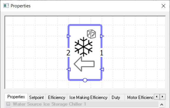
The water source ice storage chiller works in nearly the same way as the ice storage chiller does apart from the fact that the water source ice storage chiller rejects its load to a heat rejection fluid loop, rather than to the air.
This means the Water Source Ice Storage Chiller component has two loops, denoted 1 and 2 when the component is selected.
The loop denoted 1, called Loop 1, is the loop the chiller will cool (i.e. the cooling loop); while the loop denoted 2, called Loop 2, is the loop the chiller will reject heat to (i.e. the heat rejection loop).
Controllers
You can use a controller with the chiller to control how the chiller behaves.
For a chiller, the controller controls it by informing it of the amount of power the chiller should use to cool down the fluid flowing through it.
The controller does this by sending a signal, between zero and one, to the chiller dictating the proportion of the chiller’s duty it should use to cool down the fluid.
So, for example, if the chiller received a signal of zero the chiller would not cool down the fluid flowing through it. While if it received a signal of 1 the chiller will cool down the fluid flowing through it using the maximum amount of power allowed from the Duty field.
If no controller is used, the sensor used to determine the fluid’s temperature for the Setpoint field is assumed to be directly after Loop 1’s return port.
Properties
Name
This is the name of the component, it will be used in reports or error messages. You can rename components as you wish.
Description
The Description field allows the user to enter a description of the component. By default it is left blank.
Schedule
The Schedule field allows the user to apply a schedule to their component to detail the operational hours of the component.
If a schedule is applied by the user, then they should note that for all hours outside of the scheduled hours, the component will not operate.
In the case of the water source ice storage chiller, this will mean that the fluid will flow through the chiller uncooled, even if there is ice in the chiller.
The default schedule option is always on, meaning that the component will operate 24/7.
Fuel Source
With this field the user can choose the fuel source of the water source ice storage chiller.
The options provided in the drop-down menu come from the fuel sources placed in the fuel source folder. If no fuel sources have been placed in this folder, the only option available will be the “none” option.
If the “none” option is used, you will obtain a warning and the loads of the component will be discarded.
Ancillary Load Fuel Source
This option works in the same way as the Fuel Source option but allows the user to set the fuel source for the ancillary loads of the chiller.
Design Pressure Drop (1)
This field allows the user to enter the pressure drop of the fluid on Loop 1 (i.e. the cooling loop) when passing through the absorption chiller.
The drop in pressure is caused by resistance to the flow and the value entered will affect the amount of energy used by the pump on the left loop’s circuit.
If the “Not Used” option is selected for this field, the user will be asked to enter in a Capacity of the fluid loop through this component.
Design Pressure Drop (2)
This field allows the user to enter the pressure drop of the fluid on Loop 2 (i.e. the heat rejection loop) when passing through the absorption chiller.
The drop in pressure is caused by resistance to the flow and the value entered will affect the amount of energy used by the pump on the right loop’s circuit.
If the “Not Used” option is selected for this field, the user will be asked to enter in a Capacity of the fluid loop through this component.
Design Flow Delta T (1)
The Design Flow Delta T (1) field allows the user to size the flow rate of the cooling loop of the component such that the fluid flowing through the component is kept within a certain temperature band (Please note that this is the loop marked with a 1 when you click on the component).
The user can choose not to size the flow rate using this band, by choosing the “None” option. If the user decides to use this option, by choosing the “Value” option, they will need to make sure that they have a pump on the same circuit loop as the component with the pump’s Design Flow Rate field set to “Sized”.
The value entered into the Design Flow Delta T field of the chiller affects the flow rate of the circuit loop in the following way. If the component has a setpoint of \(x\) and a Design Flow Delta T of \(y\), then the fluid will always be kept within the temperature range \(x-y\) to \(x+y\) when flowing through the component by ensuring the design flow rate of the circuit is sized high enough.
If multiple components / collections on the same circuit have a Design Flow Delta T value entered, TAS will take the results of the one which requires the highest design flow rate.
Please note that for components, the Design Flow Delta T will also size the flow rate so that the demand placed on the component is also met.
Design Flow Delta T (2)
The Design Flow Delta T (2) field allows the user to size the flow rate of the heat rejection loop of the component such that the fluid flowing through the component is kept within a certain temperature band (Please note that this is the loop marked with a 2 when you click on the component).
Apart from this difference, it works in the same way as the Design Flow Delta T (1) field.
Setpoint
When a temperature is entered into the Setpoint field, the component will attempt to regulate the temperature of the fluid going through it to reach the setpoint.
In the case of the water source ice storage chiller, it will cool the fluid so it reaches the setpoint, but it will not be able to warm up the fluid to reach this setpoint. To heat the fluid you would need another component, for instance a boiler.
Please note that when a controller is used in conjunction with the chiller, the Setpoint field will disappear from the properties. This is done because the chiller is being controlled by a controller and will cool down the fluid when the controller sends a signal informing the chiller to do so.
When the Setpoint field is visible, modifiers can be added to the setpoint using the Setpoint tab.
Efficiency
Upon clicking on the Efficiency field, you will be transferred over to the Efficiency tab where you can create a profile for the efficiency of the chiller.
Normally the modifier chosen here would be a table modifier with a partload profile. The efficiency input for a chiller should be the EER.
Ice Making Efficiency
Like the Efficiency field, the Ice Making Efficiency field uses a modifier to create a Partload profile.
The efficiency entered here is the efficiency of the water source ice storage chiller when making ice.
Duty
The duty of a component is the upper limit on the amount of power a component can provide.
If, in a certain hour, the power demand on the component is greater than the duty of the component, the component will not be able to meet this demand (for a water source ice storage chiller, it means that the cooling by duty will not be able to cover the demand. If any ice is being stored, the ice will be used to attempt to meet the demand).
In TAS Systems, the demand met by a component is reported for each hour in the results section.
Currently, there are 3 options for setting the duty:
Unlimited
Sized
Value
In the duty tab, you will be able to choose these 3 options as well, but with the sized and value options you will be able to add a modifier.
Note that the “Unlimited” option which normally appears for component duty is not available for this property.
Unlimited
Unlimited means the component is always able to meet the demand. Please note that this option cannot be used when a controller is attached to the component.
Sized
Allows the user to size the duty on a design condition. The user will also be asked for a size fraction and a method to size on. With the method option, you get to choose from the following options:
Add load, all attached – TAS Systems will size the duty of the component on the demand from all attached collections in the circuit.
Add load, local – TAS systems will size the duty of the component on the demand from all collections on the same loop as the component.
Please note that to size the duty the user will need to have design conditions in their systems file.
Value
With this option the user will type in the duty of the component.
Ice Capacity
The Ice Capacity field allows the user to input the maximum amount of ice the water source ice storage chiller can store.
The user can determine how to set the capacity of the chiller from the following two options:
Sized – Allows the user to size the ice storage chiller during the simulation. An Hours at Full Load field will appear, allowing the user to enter how many hours of the chiller running at full load would it take to fully replenish the ice.
Value – With this option the user would type in the ice capacity into the software.
Initial Ice Reserve
The Initial Ice Reserve field allows the user to set the amount of stored ice the water source ice storage chiller has at the start of the simulation.
The user should enter the amount of ice stored as a percentage of the ice capacity.
Ice Melt Chiller Fraction
This field allows the user to enter in a minimum demand always met by the chiller’s duty, even when the chiller is set to prioritise cooling with ice.
This minimum demand is entered as a fraction of the duty, where zero would denote there is no minimum demand always met by the duty of the chiller.
Schedule: Cooling with Ice
This field allows the user to set a schedule dictating the hours where the chiller will prioritise cooling with Ice.
Taking into account the Ice Melt Chiller Fraction, the priority for cooling in these hours will be:
Outside of these hours, or in hours where the Cooling with Ice schedule clashes with the Making Ice schedule, the priority will be:
Schedule: Making Ice
This field allows the user to set a schedule on when the chiller will make ice.
Please be aware that outside of scheduled hours, the chiller will not cool using this functionality. Also if all of the chiller’s duty is used up meeting the Cooling demand, then the chiller will not be able to create ice.
Motor Efficiency
The Motor Efficiency field allows the user to set the chiller’s motor efficiency.
This efficiency of the motor details how efficient the chiller is at transferring the heat created due to the consumption over to the heat rejection loop.
The user enters in a percentage into this field and this percentage of the heat generated due to the consumption is transferred over to the heat rejection loop.
If the efficiency is less than 100%, some of the heat created due to the consumption will be emitted outside of the chiller rather than being transferred to the heat rejection loop.
Ancillary Load
This field allows the user to model the load used by any additional ancillary services associated with the chiller.
Any value entered here will be the associated load during any hour the chiller operates, so it is advised to make use of the modifiers available with this field.
Examples of ancillary loads which might be associated with plantroom components include internal pumps and fans which are not accounted for in the consumption figure for the component.
Modifiers can be added to this field using the Ancillary Load tab.
Air Source Heat Pump
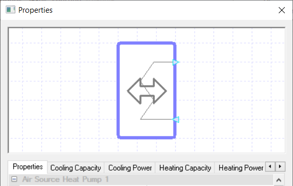
The Air Source Heat Pump component in TAS Systems allows the user to model heat pumps which transfer the load with the air.
The two ports on the side of the heat pump, which are light blue, indicate that the air source heat pump can only be connected to refrigerant circuits.
Please note that controllers cannot be used with this component.
Properties
Name
This is the name of the component, it will be used in reports or error messages. You can rename components as you wish.
Description
The Description field allows the user to enter a description of the component. By default it is left blank.
Schedule
The Schedule field allows the user to apply a schedule to their component to detail the operational hours of the component.
If a schedule is applied by the user, then they should note that for all hours outside of the scheduled hours, the component will not operate.
In the case of the air source heat pump, no heating or cooling demand from a refrigerant group would be met.
The default schedule option is always on, meaning that the component will operate 24/7.
Fuel Source
With this field the user can choose the fuel source of the air source heat pump.
The options provided in the drop-down menu come from the fuel sources placed in the fuel source folder. If no fuel sources have been placed in this folder, the only option available will be the “none” option.
If the “none” option is used, you will obtain a warning and the loads of the component will be discarded.
Fan Fuel Source
This option works in the same way as the Fuel Source option but allows the user to set the fuel source for the air source heat pump’s fan.
Ancillary Load Fuel Source
This option works in the same way as the Fuel Source option but allows the user to set the fuel source for the ancillary loads of the air source heat pump.
Type
This field allows the user to set how the air source heat pump works. There are 5 options to choose from, but only 3 should be used by the user:
Single Split
Multi Split
VRF
VRF with BC box
HVRF with BC box
Single Split
TAS models one air source heat pump for each component in the Refrigerant group. The demand and consumption figures are then worked out for each heat pump separately before being summed and reported by the Air Source Heat Pump component.
Please note that each individual heat pump has identical parameters and the parameters are the ones entered into the component.
So, for instance, if you enter the cooling duty as 1000W into the heat pump component then each individual heat pump’s cooling duty will be 1000W.
Multi Split
TAS models one air source heat pump for all components in the Refrigerant group. With a multi – split heat pump, heating and cooling cannot be provided at the same time.
This means that for an hour where there is both a heating and cooling demand, the heat pump will cater for the larger demand while not being able to meet the smaller one (TAS will inform you, with a warning, of the hours this occurs).
VRF
Like the Multi-Split option, the VRF option models one air source heat pump dealing with the load from all the components in the Refrigerant group.
The difference between the two is that the VRF option allows for both heating and cooling to be provided in a certain hour.
The VRF option keeps the refrigerant flow for heating and cooling separate. The heat pump will then meet the larger of the heating / cooling demands and heat/cool the associated refrigerant to meet it. To meet the smaller of the two demands, the heat pump will use the rejected air from the heat pump to heat/cool the refrigerant on the other refrigerant path.
To set up the VRF option correctly, TAS will ask the user to fill in the following fields:
Exchange Demand Factor (Heat)
Exchange Demand Factor (Cool)
Consumption per Port (Heat)
Consumption per Port (Cool)
Exchange Demand Factor (Heat)
When the heat pump has both a heating and cooling demand to meet with the heating demand being the bigger demand, the heat pump can attempt to meet the cooling demand by using the rejected cool air created while meeting the heating demand.
The Exchange Demand Factor (Heat) represents the extra work required to do this. The following equation states how the Exchange Demand Factor (heat) is used to work out the total demand on the heat pump, which is then used to calculate the consumption of the heat pump:
Where \(\text{Total Demand}\) is the total demand on the heat pump, \(\text{Ref Demand}\) is the absolute value of the refrigerant demand reported by the refrigerant collection (The refrigerant demand reported here is just the \(\text{Heating demand} – \text{Cooling Demand}\) ), \(\text{EDF}\) is the Exchange Demand Factor and \(\text{Cooling Demand}\) is the cooling demand reported at the refrigerant collection.
Exchange Demand Factor (Cool)
When the heat pump has both a heating and cooling demand to meet with the Cooling demand being the bigger demand, the heat pump can attempt to meet the heating demand by using the rejected hot air created while meeting the cooling demand.
The Exchange Demand Factor (Cool) represents the extra work required to do this. The following equation states how the Exchange Demand Factor (cool) is used to work out the total demand on the heat pump, which is then used to calculate the consumption of the heat pump:
Where \(\text{Total Demand}\) is the total demand on the heat pump, \(\text{Ref Demand}\) is the absolute value of the refrigerant demand reported by the refrigerant collection (The refrigerant demand reported here is just the \(\text{Heating demand} – \text{Cooling Demand}\) ), \(\text{EDF}\) is the Exchange Demand Factor and \(\text{Heating Demand}\) is the cooling demand reported at the refrigerant collection.
Consumption per Port (Heat)
This field allows the user to model additional consumption per component in the Refrigerant group connected to the heat pump which requires heating in a given hour.
The user enters a value in watts and it is multiplied by the number of components requiring heating in a given hour.
The amount is then included in the reported consumption of the chiller.
Consumption per Port (Cool)
Works in the same way as the Consumption per Port (Heat) but instead allows for additional consumption per component in the Refrigerant group connected to the heat pump which requires cooling in a given hour.
VRF with BC box
This option should only be used with Mitsubishi Heat Pumps. As Mitsubishi components are available to be imported from the manufacturer database, there is no need to use this option manually.
HVRF with BC box
This option should only be used with Mitsubishi Heat Pumps. As Mitsubishi components are available to be imported from the manufacturer database, there is no need to use this option manually.
Duty
The duty of a component is the upper limit on the amount of power a component can provide.
If, in a certain hour, the power demand on the component is greater than the duty of the component, the component will not be able to meet this demand.
In TAS Systems, the demand met by a component is reported for each hour in the results section.
The user has two methods of setting the duty of the heat pump, with the first option being “Values”. Upon choosing this option, the user is presented with the following fields:
Cooling Duty
Heating Duty
Cooling Power
Heating Power
Extra Fan Load
The second option available for setting duty of the heat pump is “sized”. Upon choosing this option, the user is presented with the following fields:
Heating: Cooling Duty Ratio
Cooling Energy Input Ratio
Cooling Efficiency
Heating Energy Input Ratio
Heating Efficiency
Fan Load : Duty Ratio
Value: Cooling Duty
The Cooling Duty field allows the user to enter in the cooling duty. This value is the upper limit on the amount of power the heat pump can provide for cooling.
Please note that the user will be able to use modifiers with this field by going to the “Cooling Capacity” tab.
Value: Heating Duty
The Heating Duty field allows the user to enter in the heating duty. This value is the upper limit on the amount of power the heat pump can provide for heating.
Please note that the user will be able to use modifiers with this field by going to the “Heating Capacity” tab.
Value: Cooling Power
The Cooling Power property is used by TAS to dictate the rate of energy consumption by the heat pump when cooling.
By default, this field has an efficiency partload profile set up (by using a modifier) which requires the user to enter the rate of energy consumption at full load as a value.
If the user deletes the modifier and doesn’t create a new one, the heat pump will always use the value entered as the consumption when the heat pump is cooling.
Value: Heating Power
The Heating Power property is used by TAS to dictate the rate of energy consumption by the heat pump when heating.
By default, this field has an efficiency partload profile set up (by using a modifier) which requires the user to enter the rate of energy consumption at full load as a value.
If the user deletes the modifier and doesn’t create a new one, the heat pump will always use the value entered as the consumption when the heat pump is heating.
Value: Extra Fan Load
The Extra Fan load property allows the user to set the consumption of the fan in the air source heat pump.
By default, this field has an efficiency partload profile set up (by using a modifier) which requires the user to enter the rate of energy consumption when the fan is at full load.
If the user deletes the modifier and doesn’t create a new one, the heat pump will always use the value entered as the consumption of the fan whenever the heat pump is heating or cooling.
Please note that consumption by the fan is included in the overall consumption of the heat pump.
When using the sizing options, please note that the options available when you choose “Value” are still visible but greyed out. This will be populated after a simulation so you can see the duties etc.
Sized: Heating: Cooling duty ratio
This field allows the user to set up a ratio between the heating duty and the cooling duty. The user will have four options to choose from:
Value – Upon choosing this option the user enters in the ratio as a value. The value the user enters will be the heating part of the ratio when the cooling side is one (So if the ratio was 3:1, the user would enter a value of 3). After sizing the heating and cooling duty’s during a simulation, TAS will modify one of the duties so that the ratio is maintained. TAS will do this so that neither duty is less than the original sized value.
Heating only - This option should only be used if the heat pump is only being used to provide heat. This option sets the cooling duty to zero, meaning the heat pump cannot provide any cooling.
Cooling only - This option should only be used if the heat pump is only being used for cooling purposes. This option sets the heating duty to zero, meaning the heat pump cannot provide any heating.
Not used - The Not Used option will not change the heating and cooling duties from the sized values taken from the simulation.
Sized: Cooling Energy Input ratio
This ratio is used to set the rate of energy consumption by the heat pump when it is cooling at its maximum cooling duty.
This value is the inverse of the cooling efficiency. The cooling efficiency field will update automatically when the user changes the cooling energy input ratio.
The ratio used is cooling power: cooling duty and the value entered is the cooling power value when the cooling duty is one (so if the cooling efficiency is 400%, the user would enter 0.25 in this field).
Please note that any modifier set in the Cooling Power Profile will be applied to the cooling power worked out by this ratio.
Sized: Cooling Efficiency
This is the cooling efficiency (cooling duty divided by cooling power) of the heat pump when it is cooling at its maximum cooling duty.
This value is the inverse of the cooling energy input ratio. The cooling energy input ratio field will update automatically when the user changes the cooling efficiency.
Sized: Heating Energy Input Ratio
This ratio is used to set the rate of energy consumption by the heat pump when it is heating at its maximum heating duty.
This value is the inverse of the heating efficiency. The heating efficiency field will update automatically when the user changes the heating energy input ratio.
The ratio used is heating power: heating duty and the value entered is the heating power value when the heating duty is one (so if the heating efficiency is 400%, the user would enter 0.25 in this field).
Please note that any modifier set in the Heating Power Profile will be applied to the Heating power worked out by this ratio.
Sized: Heating Efficiency
This is the heating efficiency (heating duty divided by heating power) of the heat pump when it is heating at its maximum heating duty.
This value is the inverse of the heating energy input ratio. The heating energy input ratio field will update automatically when the user changes the heating efficiency.
Sized: Fan Load : Duty Ratio
This ratio is used to set the rate of energy consumption by the fan in the heat pump when the fan is at full load.
The duty used in the ratio is the maximum of the Heating and Cooling duties. The value entered in this field will be the fan load part of the ratio when the duty part is one (So if the ratio was 0.3:1, the user would enter a value of 0.3 in this field).
Please note that any modifier set in the Condenser Fan Load tab will be applied to the Extra Fan Load worked out by this ratio.
Standby Power
This field sets the amount of power consumed in an hour by the heat pump when it is not being used during scheduled hours.
Ancillary Load
This field allows the user to model the load used by any additional ancillary services associated with the air source heat pump.
Any value entered here will be the associated load during any hour the heat pump operates, so it is advised to make use of the modifiers available with this field.
Examples of ancillary loads which might be associated with plantroom components include internal pumps and fans which are not accounted for in the consumption figure for the component.
Modifiers can be added to this field using the Ancillary Load tab.
Water Source Heat Pump
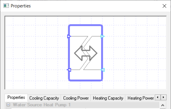
The Water Source Heat Pump component in TAS systems transfers the load from the refrigerant group to the connected fluid circuit loop.
Please note that the light blue ports are refrigerant ports and should connect up to the refrigerant group while the dark blue ports are fluid ports and should connect up to the fluid circuit loop.
Controllers cannot be used with this component.
Properties
Name
This is the name of the component, it will be used in reports or error messages. You can rename components as you wish.
Description
The Description field allows the user to enter a description of the component. By default it is left blank.
Schedule
The Schedule field allows the user to apply a schedule to their component to detail the operational hours of the component.
If a schedule is applied by the user, then they should note that for all hours outside of the scheduled hours, the component will not operate.
In the case of the water source heat pump, no heating or cooling demand from a refrigerant group would be met.
The default schedule option is always on, meaning that the component will operate 24/7.
Fuel Source
With this field the user can choose the fuel source of the water source heat pump.
The options provided in the drop-down menu come from the fuel sources placed in the fuel source folder. If no fuel sources have been placed in this folder, the only option available will be the “none” option.
If the “none” option is used, you will obtain a warning and the loads of the component will be discarded.
Ancillary Load Fuel Source
This option works in the same way as the Fuel Source option but allows the user to set the fuel source for the ancillary loads of the water source heat pump.
Design Pressure Drop
This field allows the user to enter the pressure drop of the fluid (not the refrigerant) through the component.
Please note that this is for the fluid circuit loop only, the refrigerant circuit is unaffected by this value. The drop in pressure is caused by resistance to the flow and the value entered will affect the amount of energy used by the pump on the chillers circuit.
Design Flow Delta T
The Design Flow Delta T field allows the user to size the flow rate of the circuit loop the component is on such that the fluid flowing through the component is kept within a certain temperature band (please note this is for the fluid loop, not the refrigerant loop).
The user can choose not to size the flow rate using this band, by choosing the “None” option. If the user decides to use this option, by choosing the “Value” option, they will need to make sure that they have a pump on the same circuit loop as the component with the pump’s Design Flow Rate field set to “Sized”.
The value entered into the Design Flow Delta T field of the chiller affects the flow rate of the circuit loop in the following way. If the component has a setpoint of \(x\) and a Design Flow Delta T of \(y\), then the fluid will always be kept within the temperature range \(x-y\) to \(x+y\) when flowing through the component by ensuring the design flow rate of the circuit is sized high enough.
If multiple components / collections on the same circuit have a Design Flow Delta T value entered, TAS will take the results of the one which requires the highest design flow rate.
Please note that for components, the Design Flow Delta T will also size the flow rate so that the demand placed on the component is also met.
Type
This field allows the user to set how the air source heat pump works. There are 5 options to choose from, but only 3 should be used by the user:
Single Split
Multi Split
VRF
VRF with BC box
HVRF with BC box
Single Split
TAS models one air source heat pump for each component in the Refrigerant group. The demand and consumption figures are then worked out for each heat pump separately before being summed and reported by the Air Source Heat Pump component.
Please note that each individual heat pump has identical parameters and the parameters are the ones entered into the component.
So, for instance, if you enter the cooling duty as 1000W into the heat pump component then each individual heat pump’s cooling duty will be 1000W.
Multi Split
TAS models one air source heat pump for all components in the Refrigerant group. With a multi – split heat pump, heating and cooling cannot be provided at the same time.
This means that for an hour where there is both a heating and cooling demand, the heat pump will cater for the larger demand while not being able to meet the smaller one (TAS will inform you, with a warning, of the hours this occurs).
VRF
Like the Multi-Split option, the VRF option models one air source heat pump dealing with the load from all the components in the Refrigerant group.
The difference between the two is that the VRF option allows for both heating and cooling to be provided in a certain hour.
The VRF option keeps the refrigerant flow for heating and cooling separate. The heat pump will then meet the larger of the heating / cooling demands and heat/cool the associated refrigerant to meet it. To meet the smaller of the two demands, the heat pump will use the rejected air from the heat pump to heat/cool the refrigerant on the other refrigerant path.
To set up the VRF option correctly, TAS will ask the user to fill in the following fields:
Exchange Demand Factor (Heat)
Exchange Demand Factor (Cool)
Consumption per Port (Heat)
Consumption per Port (Cool)
Exchange Demand Factor (Heat)
When the heat pump has both a heating and cooling demand to meet with the heating demand being the bigger demand, the heat pump can attempt to meet the cooling demand by using the rejected cool air created while meeting the heating demand.
The Exchange Demand Factor (Heat) represents the extra work required to do this. The following equation states how the Exchange Demand Factor (heat) is used to work out the total demand on the heat pump, which is then used to calculate the consumption of the heat pump:
Where \(\text{Total Demand}\) is the total demand on the heat pump, \(\text{Ref Demand}\) is the absolute value of the refrigerant demand reported by the refrigerant collection (The refrigerant demand reported here is just the \(\text{Heating demand} – \text{Cooling Demand}\) ), \(\text{EDF}\) is the Exchange Demand Factor and \(\text{Cooling Demand}\) is the cooling demand reported at the refrigerant collection.
Exchange Demand Factor (Cool)
When the heat pump has both a heating and cooling demand to meet with the Cooling demand being the bigger demand, the heat pump can attempt to meet the heating demand by using the rejected hot air created while meeting the cooling demand.
The Exchange Demand Factor (Cool) represents the extra work required to do this. The following equation states how the Exchange Demand Factor (cool) is used to work out the total demand on the heat pump, which is then used to calculate the consumption of the heat pump:
Where \(\text{Total Demand}\) is the total demand on the heat pump, \(\text{Ref Demand}\) is the absolute value of the refrigerant demand reported by the refrigerant collection (The refrigerant demand reported here is just the \(\text{Heating demand} – \text{Cooling Demand}\) ), \(\text{EDF}\) is the Exchange Demand Factor and \(\text{Heating Demand}\) is the cooling demand reported at the refrigerant collection.
Consumption per Port (Heat)
This field allows the user to model additional consumption per component in the Refrigerant group connected to the heat pump which requires heating in a given hour.
The user enters a value in watts and it is multiplied by the number of components requiring heating in a given hour.
The amount is then included in the reported consumption of the chiller.
Consumption per Port (Cool)
Works in the same way as the Consumption per Port (Heat) but instead allows for additional consumption per component in the Refrigerant group connected to the heat pump which requires cooling in a given hour.
VRF with BC box
This option should only be used with Mitsubishi Heat Pumps. As Mitsubishi components are available to be imported from the manufacturer database, there is no need to use this option manually.
HVRF with BC box
This option should only be used with Mitsubishi Heat Pumps. As Mitsubishi components are available to be imported from the manufacturer database, there is no need to use this option manually.
Duty
The duty of a component is the upper limit on the amount of power a component can provide.
If, in a certain hour, the power demand on the component is greater than the duty of the component, the component will not be able to meet this demand.
In TAS Systems, the demand met by a component is reported for each hour in the results section.
The user has two methods of setting the duty of the heat pump, with the first option being “Values”. Upon choosing this option, the user is presented with the following fields:
Cooling Duty
Heating Duty
Cooling Power
Heating Power
Extra Fan Load
The second option available for setting duty of the heat pump is “sized”. Upon choosing this option, the user is presented with the following fields:
Heating: Cooling Duty Ratio
Heating Efficiency
Cooling Energy Input Ratio
Cooling Efficiency
Heating Energy Input Ratio
Fan Load : Duty Ratio
Value: Cooling Duty
The Cooling Duty field allows the user to enter in the cooling duty. This value is the upper limit on the amount of power the heat pump can provide for cooling.
Please note that the user will be able to use modifiers with this field by going to the “Cooling Capacity” tab.
Value: Heating Duty
The Heating Duty field allows the user to enter in the heating duty. This value is the upper limit on the amount of power the heat pump can provide for heating.
Please note that the user will be able to use modifiers with this field by going to the “Heating Capacity” tab.
Value: Cooling Power
The Cooling Power property is used by TAS to dictate the rate of energy consumption by the heat pump when cooling.
By default, this field has an efficiency partload profile set up (by using a modifier) which requires the user to enter the rate of energy consumption at full load as a value.
If the user deletes the modifier and doesn’t create a new one, the heat pump will always use the value entered as the consumption when the heat pump is cooling.
Value: Heating Power
The Heating Power property is used by TAS to dictate the rate of energy consumption by the heat pump when heating.
By default, this field has an efficiency partload profile set up (by using a modifier) which requires the user to enter the rate of energy consumption at full load as a value.
If the user deletes the modifier and doesn’t create a new one, the heat pump will always use the value entered as the consumption when the heat pump is heating.
Value: Extra Fan Load
The Extra Fan load property allows the user to set the consumption of the fan in the air source heat pump.
By default, this field has an efficiency partload profile set up (by using a modifier) which requires the user to enter the rate of energy consumption when the fan is at full load.
If the user deletes the modifier and doesn’t create a new one, the heat pump will always use the value entered as the consumption of the fan whenever the heat pump is heating or cooling.
Please note that consumption by the fan is included in the overall consumption of the heat pump.
When using the sizing options, please note that the options available when you choose “Value” are still visible but greyed out. This will be populated after a simulation so you can see the duties etc.
Sized: Heating: Cooling duty ratio
This field allows the user to set up a ratio between the heating duty and the cooling duty. The user will have four options to choose from:
Value – Upon choosing this option the user enters in the ratio as a value. The value the user enters will be the heating part of the ratio when the cooling side is one (So if the ratio was 3:1, the user would enter a value of 3). After sizing the heating and cooling duty’s during a simulation, TAS will modify one of the duties so that the ratio is maintained. TAS will do this so that neither duty is less than the original sized value.
Heating only - This option should only be used if the heat pump is only being used to provide heat. This option sets the cooling duty to zero, meaning the heat pump cannot provide any cooling.
Cooling only - This option should only be used if the heat pump is only being used for cooling purposes. This option sets the heating duty to zero, meaning the heat pump cannot provide any heating.
Not used - The Not Used option will not change the heating and cooling duties from the sized values taken from the simulation.
Sized: Cooling Energy Input ratio
This ratio is used to set the rate of energy consumption by the heat pump when it is cooling at its maximum cooling duty.
This value is the inverse of the cooling efficiency. The cooling efficiency field will update automatically when the user changes the cooling energy input ratio.
The ratio used is cooling power: cooling duty and the value entered is the cooling power value when the cooling duty is one (so if the cooling efficiency is 400%, the user would enter 0.25 in this field).
Please note that any modifier set in the Cooling Power Profile will be applied to the cooling power worked out by this ratio.
Sized: Cooling Efficiency
This is the cooling efficiency (cooling duty divided by cooling power) of the heat pump when it is cooling at its maximum cooling duty.
This value is the inverse of the cooling energy input ratio. The cooling energy input ratio field will update automatically when the user changes the cooling efficiency.
Sized: Heating Energy Input Ratio
This ratio is used to set the rate of energy consumption by the heat pump when it is heating at its maximum heating duty.
This value is the inverse of the heating efficiency. The heating efficiency field will update automatically when the user changes the heating energy input ratio.
The ratio used is heating power: heating duty and the value entered is the heating power value when the heating duty is one (so if the heating efficiency is 400%, the user would enter 0.25 in this field).
Please note that any modifier set in the Heating Power Profile will be applied to the Heating power worked out by this ratio.
Sized: Heating Efficiency
This is the heating efficiency (heating duty divided by heating power) of the heat pump when it is heating at its maximum heating duty.
This value is the inverse of the heating energy input ratio. The heating energy input ratio field will update automatically when the user changes the heating efficiency.
Sized: Fan Load : Duty Ratio
This ratio is used to set the rate of energy consumption by the fan in the heat pump when the fan is at full load.
The duty used in the ratio is the maximum of the Heating and Cooling duties. The value entered in this field will be the fan load part of the ratio when the duty part is one (So if the ratio was 0.3:1, the user would enter a value of 0.3 in this field).
Please note that any modifier set in the Condenser Fan Load tab will be applied to the Extra Fan Load worked out by this ratio.
Standby Power
This field sets the amount of power consumed in an hour by the heat pump when it is not being used during scheduled hours.
Ancillary Load
This field allows the user to model the load used by any additional ancillary services associated with the air source heat pump.
Any value entered here will be the associated load during any hour the heat pump operates, so it is advised to make use of the modifiers available with this field.
Examples of ancillary loads which might be associated with plantroom components include internal pumps and fans which are not accounted for in the consumption figure for the component.
Modifiers can be added to this field using the Ancillary Load tab.
Water to Water Heat Pump
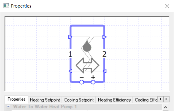
The water to water heat pump allows the user to connect a heat pump up to fluid collections, like heating and cooling collections, rather than to refrigerant collections.
Please note that the water to water heat pump should only be connected to either a heating collection or a cooling collection, as connecting it to both may cause issues when there is a heating and cooling demand in the same hour.
The water to water heat pump connects up to two fluid loops, denoted 1 and 2 when the component is selected. The loop denoted 1, called Loop 1, is the loop heat will be rejected to. The loop denoted 2, called Loop 2, is the loop that will be heated or cooled by the heat pump.
Controllers
The water to water heat pump can be used in conjunction with a controller, to control the heat pump.
If a controller is connected to the plus signal port, then the signal from the controller is the proportion of the heat pump’s heating duty it should use to heat the fluid.
If a controller is connected to the minus signal port, then the signal from the controller is the proportion of the heat pump’s cooling duty it should use to cool the fluid.
If no controller is used, the sensor used to determine the fluid’s temperature for the Setpoint fields is assumed to be directly after the return port on Loop 2.
Properties
Name
This is the name of the component, it will be used in reports or error messages. You can rename components as you wish.
Description
The Description field allows the user to enter a description of the component. By default it is left blank.
Schedule
The Schedule field allows the user to apply a schedule to their component to detail the operational hours of the component.
If a schedule is applied by the user, then they should note that for all hours outside of the scheduled hours, the component will not operate.
In the case of the water to water heat pump, no heating or cooling demand would be met.
The default schedule option is always on, meaning that the component will operate 24/7.
Fuel Source
With this field the user can choose the fuel source of the water to water heat pump.
The options provided in the drop-down menu come from the fuel sources placed in the fuel source folder. If no fuel sources have been placed in this folder, the only option available will be the “none” option.
If the “none” option is used, you will obtain a warning and the loads of the component will be discarded.
Ancillary Load Fuel Source
This option works in the same way as the Fuel Source option but allows the user to set the fuel source for the ancillary loads of the water source heat pump.
Design Pressure Drop (1)
This field allows the user to enter the pressure drop of the fluid on Loop 1 (i.e. the heat rejection loop) when flowing through the component.
The drop in pressure is caused by resistance to the flow and the value entered will affect the amount of energy used by the pump on the left loop’s circuit.
If the “Not Used” option is selected for this field, the user will be asked to enter in a Capacity for the fluid loop through this component.
Design Pressure Drop (2)
This field allows the user to enter the pressure drop of the fluid on Loop 2 (i.e. the heating / cooling loop) when flowing through the component.
The drop in pressure is caused by resistance to the flow and the value entered will affect the amount of energy used by the pump on the left loop’s circuit.
If the “Not Used” option is selected for this field, the user will be asked to enter in a Capacity for the fluid loop through this component.
Design Flow Delta T (1)
This field allows the user to size the flow rate of the heat rejection loop of the component such that the fluid flowing through the component is kept within a certain temperature band (Please note that this is the loop marked with a 1 when you click on the component).
The user can choose not to size the flow rate using this band, by choosing the “None” option.
If the user decides to use this option, by choosing the “Value” option, they will need to make sure that they have a pump on the same circuit loop as the component with the pump’s Design Flow Rate field set to “Sized”.
The value entered into the Design Flow Delta T field affects the flow rate of the circuit loop in the following way. If the component has a setpoint of x and a Design Flow Delta T of y, then the fluid will always be kept within the temperature range \(x-y\) to \(x+y\) when flowing through the component by ensuring the design flow rate of the circuit is sized high enough.
If multiple components / collections on the same circuit have a Design Flow Delta T value entered, TAS will take the results of the one which requires the highest design flow rate.
Please note that for components, the Design Flow Delta T will also size the flow rate so that the demand placed on the component is also met.
Design Flow Delta T (2)
The Design Flow Delta T (2) field works in the same way as the Design Flow Delta T (1) field, which is described above, but affects the heating/cooling loop instead of Loop 1. I.e. the loop marked with a 2 when you click on the component.
Please read the description of the Design Flow Delta T (1) field for how this works.
Heating Setpoint
When a temperature is entered into the Heating Setpoint field, the component will attempt to regulate the temperature of the fluid going through it to reach the setpoint.
In the case of the water to water heat pump, it will heat the fluid so it reaches the heating setpoint.
Please note that when a controller is used in conjunction with the water to water heat pump, the Heating Setpoint field will disappear from the properties. This is done because the water to water heat pump is being controlled by a controller and will heat the fluid when the controller sends a signal informing the water to water heat pump to do so.
When the Heating Setpoint field is visible, modifiers can be added to the setpoint using the Heating Setpoint tab.
Cooling Setpoint
When a temperature is entered into the Cooling Setpoint field, the component will attempt to regulate the temperature of the fluid going through it to reach the setpoint.
In the case of the water to water heat pump, it will cool the fluid so it reaches the cooling setpoint.
Please note that when a controller is used in conjunction with the water to water heat pump, the Cooling Setpoint field will disappear from the properties. This is done because the water to water heat pump is being controlled by a controller and will cool the fluid when the controller sends a signal informing the water to water heat pump to do so.
When the Cooling Setpoint field is visible, modifiers can be added to the setpoint using the Cooling Setpoint tab.
Heating Efficiency
Upon clicking on the Heating Efficiency field, you will be transferred over to the Heating Efficiency tab where you can create a profile for the heating efficiency of the water to water heat pump.
Normally the modifier chosen here would be a table modifier with a partload profile.
Cooling Efficiency
Upon clicking on the Cooling Efficiency field, you will be transferred over to the Cooling Efficiency tab where you can create a profile for the cooling efficiency of the water to water heat pump.
Normally the modifier chosen here would be a table modifier with a partload profile.
The cooling efficiency input for a heat pump should be the EER.
Heating Duty
The heating duty of a component is the upper limit on the amount of power a component can provide for heating.
If, in a certain hour, the power demand on the component is greater than the duty of the component, the component will not be able to meet this demand (For a water to water heat pump, if the heating demand is bigger than the heating duty it means that the heat pump will not be able to cover the heating demand.).
In TAS Systems, the demand met by a component is reported for each hour in the results section. Currently, there are 3 options for setting the duty:
Unlimited
Sized
Value
In the Heating Duty tab, you will be able to choose these 3 options as well, but with the sized and value options you will be able to add a modifier.
Unlimited
Unlimited means the component is always able to meet the demand. Please note that this option cannot be used when a controller is attached to the component.
Sized
Allows the user to size the duty on a design condition. The user will also be asked for a size fraction and a method to size on.
With the method option, you get to choose from the following options:
Add load, all attached - TAS Systems will size the duty of the component on the demand from all attached collections in the circuit.
Add load, local - TAS systems will size the duty of the component on the demand from all collections on the same loop as the component.
Please note that to size the duty the user will need to have design conditions in their systems file.
When using the “Sized” option the user also has the option to include or exclude storage losses from the sizing calculation. This is used to account for (or ignore) the additional load due to a Tank component in the same system.
Value
With this option the user will type in the heating duty of the component.
Cooling Duty
The cooling duty of a component is the upper limit on the amount of power a component can provide.
If, in a certain hour, the power demand on the component is greater than the duty of the component, the component will not be able to meet this demand (For a water to water heat pump, if the cooling demand is bigger than the cooling duty it means that the heat pump will not be able to cover the cooling demand.).
In TAS Systems, the demand met by a component is reported for each hour in the results section. Currently, there are 3 options for setting the duty:
Unlimited
Sized
Value
In the Cooling Duty tab, you will be able to choose these 3 options as well, but with the sized and value options you will be able to add a modifier.
Unlimited
Unlimited means the component is always able to meet the demand. Please note that this option cannot be used when a controller is attached to the component.
Sized
Allows the user to size the duty on a design condition. The user will also be asked for a size fraction and a method to size on.
With the method option, you get to choose from the following options:
Add load, all attached - TAS Systems will size the duty of the component on the demand from all attached collections in the circuit.
Add load, local - TAS systems will size the duty of the component on the demand from all collections on the same loop as the component.
Please note that to size the duty the user will need to have design conditions in their systems file.
When using the “Sized” option the user also has the option to include or exclude storage losses from the sizing calculation. This is used to account for (or ignore) the additional load due to a Tank component in the same system.
Value
With this option the user will type in the cooling duty of the component.
Motor Efficiency
The Motor Efficiency field allows the user to set the chiller’s motor efficiency.
This efficiency of the motor details how efficient the chiller is at transferring the heat created due to the consumption over to the heat rejection loop.
The user enters in a percentage into this field and this percentage of the heat generated due to the consumption is transferred over to the heat rejection loop. If the efficiency is less than 100%, some of heat created due to the consumption will be emitted outside of the chiller rather than being transferred to the heat rejection loop.
For example, if the Motor Efficiency is 85%, this implies that 15% of the energy associated with the chiller consumption is expended outside the chiller, and 85% becomes heat within the chiller itself (and this heat is added to the heat rejection loop).
Ancillary Load
This field allows the user to model the load used by any additional ancillary services associated with the water to water heat pump.
Any value entered here will be the associated load during any hour the heat pump operates, so it is advised to make use of the modifiers available with this field.
Examples of ancillary loads which might be associated with plantroom components include internal pumps and fans which are not accounted for in the consumption figure for the component.
Modifiers can be added to this field using the Ancillary Load tab.
Four Pipe Heat Pump
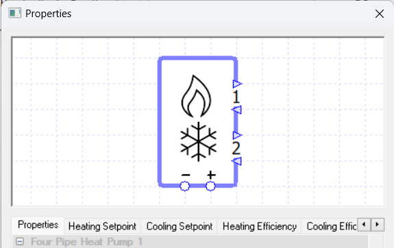
The four pipe heat pump allows the user to provide hot water and cold water from the same source. When there is both a heating and a cooling demand, heat can be transferred between the two loops more efficiently than providing the heating and cooling separately.
The loop indicated by the number 1 is for heating.
The loop indicated by the number 2 is for cooling.
Controllers
The four pipe heat pump can be used in conjunction with a controller.
If a controller is connected to the plus signal port, then the signal from the controller is the proportion of the heat pump’s heating duty it should use to heat the fluid.
If a controller is connected to the minus signal port, then the signal from the controller is the proportion of the heat pump’s cooling duty it should use to cool the fluid.
If no controller is used, the sensor used to determine the fluid’s temperature for the Setpoint fields is assumed to be directly after the return port on loop 1 (for heating) or loop 2 (for cooling).
Properties
Name
This is the name of the component, it will be used in reports or error messages. You can rename components as you wish.
Description
The Description field allows the user to enter a description of the component. By default it is left blank.
Schedule
The Schedule field allows the user to apply a schedule to their component to detail the operational hours of the component.
If a schedule is applied by the user, then they should note that for all hours outside of the scheduled hours, the component will not operate.
In the case of the four pipe heat pump, no heating or cooling demand would be met.
The default schedule option is always on, meaning that the component will operate 24/7.
Fuel Source
With this field the user can choose the fuel source of the four pipe heat pump.
The options provided in the drop-down menu come from the fuel sources placed in the fuel source folder. If no fuel sources have been placed in this folder, the only option available will be the “none” option.
If the “none” option is used, you will obtain a warning and the loads of the component will be discarded.
Ancillary Load Fuel Source
This option works in the same way as the Fuel Source option but allows the user to set the fuel source for the ancillary loads of the four pipe heat pump.
Design Pressure Drop (1)
This field allows the user to enter the pressure drop of the fluid on Loop 1 (i.e. the heating loop) when flowing through the component.
The drop in pressure is caused by resistance to the flow and the value entered will affect the amount of energy used by the pump on the heating circuit.
If the “Not Used” option is selected for this field, the user will be asked to enter in a Capacity for the fluid loop through this component.
Design Pressure Drop (2)
This field allows the user to enter the pressure drop of the fluid on Loop 2 (i.e. the cooling loop) when flowing through the component.
The drop in pressure is caused by resistance to the flow and the value entered will affect the amount of energy used by the pump on the cooling circuit.
If the “Not Used” option is selected for this field, the user will be asked to enter in a Capacity for the fluid loop through this component.
Design Flow Delta T (1)
This field allows the user to size the flow rate of Loop 1 (i.e. the heating loop) of the component such that the fluid flowing through the component is kept within a certain temperature band (Please note that this is the loop marked with a 1 when you click on the component).
The user can choose not to size the flow rate using this band, by choosing the “None” option.
If the user decides to use this option, by choosing the “Value” option, they will need to make sure that they have a pump on the same circuit loop as the component with the pump’s Design Flow Rate field set to “Sized”.
The value entered into the Design Flow Delta T field affects the flow rate of the circuit loop in the following way. If the component has a setpoint of x and a Design Flow Delta T of y, then the fluid will always be kept within the temperature range \(x-y\) to \(x+y\) when flowing through the component by ensuring the design flow rate of the circuit is sized high enough.
If multiple components / collections on the same circuit have a Design Flow Delta T value entered, TAS will take the results of the one which requires the highest design flow rate.
Please note that for components, the Design Flow Delta T will also size the flow rate so that the demand placed on the component is also met.
Design Flow Delta T (2)
The Design Flow Delta T (2) field works in the same way as the Design Flow Delta T (1) field, which is described above, but affects Loop 2 (i.e., the cooling loop) instead of Loop 1 (i.e., the heating loop). Loop 2 is the loop marked with a 2 when you click on the component.
Please read the description of the Design Flow Delta T (1) field for how this works.
Heating Setpoint
When a temperature is entered into the Heating Setpoint field, the component will attempt to regulate the temperature of the fluid going through it to reach the setpoint.
In this case, the four pipe heat pump will heat the fluid so it reaches the Heating Setpoint.
Please note that when a controller is used in conjunction with the four pipe heat pump, the Heating Setpoint field will disappear from the properties. This is done because the four pipe heat pump is being controlled by a controller and will heat the fluid when the controller sends a signal informing the four pipe heat pump to do so.
When the Heating Setpoint field is visible, modifiers can be added to the setpoint using the Heating Setpoint tab.
Cooling Setpoint
When a temperature is entered into the Cooling Setpoint field, the component will attempt to regulate the temperature of the fluid going through it to reach the setpoint.
In this case, the four pipe heat pump will cool the fluid so it reaches the Cooling Setpoint.
Please note that when a controller is used in conjunction with the four pipe heat pump, the Cooling Setpoint field will disappear from the properties. This is done because the four pipe heat pump is being controlled by a controller and will heat the fluid when the controller sends a signal informing the four pipe heat pump to do so.
When the Cooling Setpoint field is visible, modifiers can be added to the setpoint using the Cooling Setpoint tab.
Exchange Demand Factor (Heat)
When the heat pump has both a heating and cooling demand to meet with the heating demand being the bigger demand, the heat pump can transfer rejected heat from the cooling loop to the heating loop.
The Exchange Demand Factor (Heat) represents the extra work required to do this, for cases when the heating demand exceeds the cooling demand. The following equation shows how the Exchange Demand Factor (heat) is used to work out the total demand on the heat pump, which is then used to calculate the consumption of the heat pump:
Where \(\text{Total Demand}\) is the total demand on the heat pump, \(\text{Net Demand} = \text{Heating demand} – \text{Cooling Demand}\), and \(\text{EDF}\) is the Exchange Demand Factor.
Exchange Demand Factor (Cool)
When the heat pump has both a heating and cooling demand to meet with the cooling demand being the bigger demand, the heat pump can transfer rejected heat from the cooling loop to the heating loop.
The Exchange Demand Factor (Cool) represents the extra work required to do this, for cases when the cooling demand exceeds the heating demand. The following equation shows how the Exchange Demand Factor (cool) is used to work out the total demand on the heat pump, which is then used to calculate the consumption of the heat pump:
Where \(\text{Total Demand}\) is the total demand on the heat pump, \(\text{Net Demand} = \text{Cooling demand} – \text{Heating Demand}\), and \(\text{EDF}\) is the Exchange Demand Factor.
Heating Efficiency
Upon clicking on the Heating Efficiency field, you will be transferred over to the Heating Efficiency tab where you can create a profile for the heating efficiency of the four pipe heat pump.
Normally the modifier chosen here would be a table modifier with a partload profile.
Cooling Efficiency
Upon clicking on the Cooling Efficiency field, you will be transferred over to the Cooling Efficiency tab where you can create a profile for the cooling efficiency of the four pipe heat pump.
Normally the modifier chosen here would be a table modifier with a partload profile.
Heating Duty
The heating duty of a component is the upper limit on the amount of power a component can provide for heating.
If, in a certain hour, the power demand on the component is greater than the duty of the component, the component will not be able to meet this demand (For a four pipe heat pump, if the heating demand is bigger than the heating duty it means that the heat pump will not be able to cover the heating demand.).
In TAS Systems, the demand met by a component is reported for each hour in the results section. Currently, there are 3 options for setting the duty:
Unlimited
Sized
Value
In the Heating Duty tab, you will be able to choose these 3 options as well, but with the sized and value options you will be able to add a modifier.
Unlimited
Unlimited means the component is always able to meet the demand. Please note that this option cannot be used when a controller is attached to the component.
Sized
Allows the user to size the duty on a design condition. The user will also be asked for a size fraction and a method to size on.
With the method option, you get to choose from the following options:
Add load, all attached - TAS Systems will size the duty of the component on the demand from all attached collections in the circuit.
Add load, local - TAS systems will size the duty of the component on the demand from all collections on the same loop as the component.
Please note that to size the duty the user will need to have design conditions in their systems file.
When using the “Sized” option the user also has the option to include or exclude storage losses from the sizing calculation. This is used to account for (or ignore) the additional load due to a Tank component in the same system.
Value
With this option the user will type in the heating duty of the component.
Cooling Duty
The cooling duty of a component is the upper limit on the amount of power a component can provide.
If, in a certain hour, the power demand on the component is greater than the duty of the component, the component will not be able to meet this demand (For a four pipe heat pump, if the cooling demand is bigger than the cooling duty it means that the heat pump will not be able to cover the cooling demand.).
In TAS Systems, the demand met by a component is reported for each hour in the results section. Currently, there are 3 options for setting the duty:
Unlimited
Sized
Value
In the Cooling Duty tab, you will be able to choose these 3 options as well, but with the sized and value options you will be able to add a modifier.
Unlimited
Unlimited means the component is always able to meet the demand. Please note that this option cannot be used when a controller is attached to the component.
Sized
Allows the user to size the duty on a design condition. The user will also be asked for a size fraction and a method to size on.
With the method option, you get to choose from the following options:
Add load, all attached - TAS Systems will size the duty of the component on the demand from all attached collections in the circuit.
Add load, local - TAS systems will size the duty of the component on the demand from all collections on the same loop as the component.
Please note that to size the duty the user will need to have design conditions in their systems file.
When using the “Sized” option the user also has the option to include or exclude storage losses from the sizing calculation. This is used to account for (or ignore) the additional load due to a Tank component in the same system.
Value
With this option the user will type in the cooling duty of the component.
Ancillary Load
This field allows the user to model the load used by any additional ancillary services associated with the four pipe heat pump.
Any value entered here will be the associated load during any hour the heat pump operates, so it is advised to make use of the modifiers available with this field.
Examples of ancillary loads which might be associated with plantroom components include internal pumps and fans which are not accounted for in the consumption figure for the component.
Modifiers can be added to this field using the Ancillary Load tab.
Cooling Tower
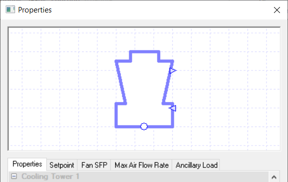
The Cooling Tower component in TAS Systems allows the user to model a fan driven cooling tower in TAS Systems.
The cooling tower rejects heat by passing the fluid through a moving air stream.
Controllers
Controllers can be used with the cooling tower to control it by informing it of the amount of air flow the fans should provide to facilitate the heat exchange.
The controller does this by sending a signal, between zero and one, to the cooling tower dictating the proportion of the cooling tower’s max air flow rate it should use to cool down the fluid.
So, for example, if the cooling tower received a signal of zero then the fans will be switched off for the whole hour. While if it received a signal of 1 the cooling tower’s fans would provide the maximum flow rate specified in the Max Air Flow Rate field.
If no controller is used, the sensor used to determine the fluid’s temperature for the Cooling Setpoint field is assumed to be directly after the return port of the cooling tower.
Properties
Name
This is the name of the component, it will be used in reports or error messages. You can rename components as you wish.
Description
The Description field allows the user to enter a description of the component. By default it is left blank.
Schedule
The Schedule field allows the user to apply a schedule to their component to detail the operational hours of the component.
If a schedule is applied by the user, then they should note that for all hours outside of the scheduled hours, the component will not operate.
In the case of the cooling tower, this will mean that the fluid will flow through the cooling tower uncooled, as the cooling tower fans will not operate.
The default schedule option is always on, meaning that the component will operate 24/7.
Fan Fuel Source
With this field the user can choose the fuel source of the cooling tower’s fans.
The options provided in the drop-down menu come from the fuel sources placed in the fuel source folder. If no fuel sources have been placed in this folder, the only option available will be the “none” option.
If the “none” option is used, you will obtain a warning and the loads of the component will be discarded.
Ancillary Load Fuel Source
This option works in the same way as the Fuel Source option but allows the user to set the fuel source for the ancillary loads of the cooling tower.
Design Pressure Drop
This field allows the user to enter the pressure drop of the fluid through the component.
The drop in pressure is caused by resistance to the flow and the value entered will affect the amount of energy used by the pump on this circuit.
If the “Not Used” option is selected for this field, the user will be asked to enter in a Capacity for the fluid loop through this component.
Cooling Setpoint
When a temperature is entered into the Cooling Setpoint field, the component will attempt to regulate the temperature of the fluid going through it by cooling the fluid to reach this setpoint.
It should be noted that the cooling tower will not always be able to meet this setpoint. For instance if the cooling setpoint of the cooling tower is set to lower than the external wet bulb temperature for a given hour then the cooling tower will only be able to cool the fluid down to the external wetbulb temperature in this hour.
Please note that when a controller is used in conjunction with the cooling tower, the Cooling Setpoint field will disappear from the properties. This is done because the cooling tower is being controlled by a controller rather than being controlled using this setpoint field.
When the Setpoint field is visible, modifiers can be added to the setpoint using the Cooling Setpoint tab.
Minimum Approach
When the temperature difference between the fluid the cooling tower is cooling and the external wet bulb temperature is very small, the cooling tower will become very inefficient at rejecting heat.
To get around this problem, the user can enter a minimum approach, which creates a buffer zone to prevent inefficient operation.
The minimum approach works in the following way. If the user enters the value \(x\) into this field, then when the air’s wet-bulb temperature is within \(x\) of the cooling setpoint of the cooling tower or when the cooling setpoint of the cooling tower is above the external wetbulb temperature, TAS will set the cooling setpoint to:
Please note that depending on the properties of the cooling tower, it may not always be able to meet this revised setpoint.
Variable Speed Fans
This tick box field allows the user to decide on how the fans in the cooling tower work.
If this field is left un-ticked, the air flow rates entered in the Max Air Flow Rate field and the Min Air Flow Rate field are the only air flow rates the fans can provide. As the fans can’t provide any other flow rate, they alternate between the two air flow rates to cover partial loads.
If this field is ticked, the Fans can provide any air flow rate between the max air flow rate (which will be the maximum allowed air flow) and the min air flow rate (which will be the minimum allowed air flow).
Allowing the fans to be variable provides better performances at part loads.
Please note that for both options, if the cooling tower has a partial load which requires an air flow rate below the minimum air flow rate, the cooling tower will meet this by turning the fan on and off.
Also note that TAS Systems reports the average air flow rate for the hour in its result section which means, for instance, the reported air flow rate for the hour can be less than the minimum air flow rate.
Fan SFP
The Fan SFP field allows the user to enter the SFP of the cooling tower’s fans. By default the fan has a modifier profile set up in the Fan SFP tab and the user only needs to enter the SFP at the fan’s full load.
Heat Transfer Coefficient
This field allows the user to input the heat transfer coefficient for the heat exchange between the air and water flows.
Heat Transfer Surface Area
This field allows the user to input the surface area where heat transfer can occur between the air and water flows.
This surface area can be set using two different methods.
If the Value option is selected, then the user will be asked to enter in the heat transfer surface area.
If the Sized option is selected, then the heat transfer surface area will be sized based on design conditions entered into the cooling tower properties.
These design conditions will be discussed in their own property fields as they can also be used for sizing the max air flow rate.
Please note that a size fraction also appears, allowing the area to be oversized or undersized.
Max Air Flow Rate
The Max Air Flow Rate field allows the user to specify the maximum permitted air flow through the cooling tower.
Please note that how this maximum is used varies depending on the choice made for the Variable Speed Fans field.
Depending on other properties, there are three options to choose from when setting the Max Air Flow Rate:
Value
Fan Load Ratio
Air Flow/ Water Flow Ratio
Value
Upon Choosing the Value option the user is asked to enter the max air flow rate. This option is the default option and is always available.
Modifiers can be used with this field by going to the Max Air Flow Rate field. By default, a modifier is already applied to this field.
Fan Load Ratio
This option is only available when the Heat Transfer Surface Area field is sized, as it will make use of the design condition options that appear when that field is sized.
Upon choosing the Fan Load Ratio option, a Fan Load Ratio field will appear asking the user to enter in the ratio of the maximum fan load to the maximum cooling load.
Air Flow / Water Flow Ratio
This option is only available when the Heat Transfer Surface Area field is sized, as it will make use of the design condition options that appear when that field is sized.
Upon choosing this option, an Air Flow / Water Flow Ratio field will appear asking the user to enter the ratio of the maximum air flow rate to the maximum fluid flow rate.
Min Air Flow Rate
The Min Air Flow Rate field allows the user to specify the minimum permitted air flow the cooling tower fans can provide.
Please note that how this minimum is used varies depending on the choice made for the Variable Speed Fans field. How the minimum air flow rate is set depends on how the max air flow rate is calculated.
If the Max Air Flow Rate field is set to “Value” then the user will be required to enter in the minimum air flow rate into this field.
If the Max Air Flow Rate field is not set to “Value”, however, then the user will be required to enter in the minimum air flow sizing ratio into the Min Air Flow Sizing Ratio field. This ratio would be the ratio between the minimum air flow rate and the maximum air flow rate.
Design Water Flow Rate
This field is only available when the Heat Transfer Surface Area field is sized and sets the flow rate of the water entering the cooling tower on the design condition.
There are two options to choose from when using this field:
Value - With this option the user must enter in the water flow rate to be used on the sizing condition.
As Pump Design Flow Rate - With this option the design flow rate from the pump on the heat rejection loop will be used in the design conditions.
Design External Wetbulb
This field is only available when the Heat Transfer Surface Area field is sized and sets the external wetbulb temperature used on the design condition.
There are three options to choose from with this field:
Value - Upon choosing this option, the user would enter the design external wetbulb temperature as a value.
Peak External - Upon choosing this option, TAS will take the peak external wet bulb temperature from the weather data as the design external wetbulb for the sizing run.
Max Operating - Upon choosing this option, the user is asked to enter a limiting wetbulb temperature. TAS will then compare this temperature with the peak external wetbulb temperature from the weather data and use the minimum value as the design external wetbulb temperature.
Design Approach
This field is only available when the Heat Transfer Surface Area field is sized and sets the minimum approach used on the design conditions.
Design Range
This field is only available when the Heat Transfer Surface Area field is sized and sets the water temperature drop of the fluid flowing through the cooling tower used on the design conditions.
Drift Loss at Max Air Flow
The Drift Loss at Max Air Flow field allows the user to enter the proportion of the water flow lost due to water droplets being carried out with the exhaust air.
The percentage entered in this field will be the percentage loss when the air flow is at its maximum rate. As the air flow rate decreases, the drift loss percentage will decrease linearly as well.
Blowdown Concentration Ratio
The Blowdown Concentration Ratio field is used to calculate the amount of blowdown.
As some of the water in the cooling tower evaporates, the concentration of impurities in the cooling tower water will increase. To maintain the concentration within acceptable levels, some of the cooling tower water is rejected (which is called blowdown) and replaced with fresh water. In this field the user is required to enter the ratio:
To enter the ratio into this field, the user will enter the value \(x\), where the ratio is \(1:x\).
TAS will then use this ratio to maintain the impurity concentration of the cooling tower water, any water added to the cooling tower will be reported in the results under the make-up water column.
Ancillary Load
This field allows the user to model the load used by any additional ancillary services associated with the cooling tower.
Any value entered here will be the associated load during any hour the heat pump operates, so it is advised to make use of the modifiers available with this field.
Examples of ancillary loads which might be associated with plantroom components include internal pumps and fans which are not accounted for in the consumption figure for the component.
Modifiers can be added to this field using the Ancillary Load tab.
Dry Cooler
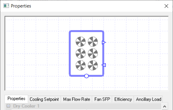
A dry cooler is a heat rejection component which rejects heat from the fluid entering it to the outside air.
Controllers
Controllers can be used with the dry cooler to control it by informing it of the amount of air flow the fans should provide to facilitate the heat exchange.
The controller does this by sending a signal, between zero and one, to the dry cooler dictating the proportion of the dry cooler’s max air flow rate it should use to cool down the fluid.
So, for example, if the dry cooler received a signal of zero then the fans will be switched off for the whole hour. While if it received a signal of 1 the dry cooler’s fans would provide the maximum flow rate specified in the Max Air Flow Rate field.
If no controller is used, the sensor used to determine the fluid’s temperature for the Cooling Setpoint field is assumed to be directly after the return port of the dry cooler.
Properties
Name
This is the name of the component, it will be used in reports or error messages. You can rename components as you wish.
Description
The Description field allows the user to enter a description of the component. By default it is left blank.
Fan Fuel Source
With this field the user can choose the fuel source of the dry cooler’s fans.
The options provided in the drop-down menu come from the fuel sources placed in the fuel source folder. If no fuel sources have been placed in this folder, the only option available will be the “none” option.
If the “none” option is used, you will obtain a warning and the loads of the component will be discarded.
Ancillary Load Fuel Source
This option works in the same way as the Fuel Source option but allows the user to set the fuel source for the ancillary loads of the dry cooler.
Design Pressure Drop
This field allows the user to enter the pressure drop of the fluid when passing through the component.
The drop in pressure is caused by resistance to the flow and the value entered will affect the amount of energy used by the pump on this circuit.
If the “Not Used” option is selected for this field, the user will be asked to enter in a Capacity for the fluid loop through this component.
Cooling Setpoint
When a temperature is entered into the Cooling Setpoint field, the component will attempt to regulate the temperature of the fluid going through it by cooling the fluid to reach this setpoint.
It should be noted that the dry cooler will not always be able to meet this setpoint. For instance if the cooling setpoint of the dry cooler is set to lower than the external drybulb temperature for a given hour then the dry cooler will only be able to cool the fluid down to the external drybulb temperature in this hour.
Please note that when a controller is used in conjunction with the dry cooler, the Cooling Setpoint field will disappear from the properties. This is done because the dry cooler is being controlled by a controller rather than being controlled using this setpoint field.
When the Setpoint field is visible, modifiers can be added to the setpoint using the Cooling Setpoint tab.
Variable Speed Fans
This tick box field allows the user to decide on how the fans in the dry cooler work.
If this field is left un-ticked, the air flow rates entered in the Max Air Flow Rate field and the Min Air Flow Rate field are the only air flow rates the fans can provide. As the fans can’t provide any other flow rate, they alternate between the two air flow rates to cover partial loads.
If this field is ticked, the fans can provide any air flow rate between the max air flow rate (which will be the maximum allowed air flow) and the min air flow rate (which will be the minimum allowed air flow).
Allowing the fans to be variable provides better performances at part loads.
Please note that for both options, if the dry cooler has a partial load which requires an air flow rate below the minimum air flow rate, the dry cooler will meet this by turning the fan on and off.
Also note that TAS Systems reports the average air flow rate for the hour in its result section which means, for instance, the reported air flow rate for the hour can be less than the minimum air flow rate.
Fan SFP
The Fan SFP field allows the user to enter the SFP of the dry cooler’s fans. Modifiers can be applied to this field by going to the Fan SFP tab.
Calculation Method
In TAS systems, there are two options to calculate the maximum rate of heat rejection for the dry cooler:
Efficiency
NTU Method
Efficiency
The first calculation method is efficiency. Upon choosing this option the user is asked to enter the efficiency of the dry cooler.
The efficiency of the dry cooler is calculated by the following formula:
Where \(T_\text{out}\) is the temperature of the fluid leaving the dry cooler, \(T_\text{in}\) is the temperature of the fluid entering the dry cooler and \(T_\text{db ext}\) is the external dry bulb temperature.
NTU Method
The second calculation method is the NTU method. Upon choosing this method, the user will need to input: The heat transfer surface area, the heat transfer coefficient and the Exchanger type.
After entering these details, TAS will then work out the rate of heat transfer of the Exchanger.
Max Air Flow Rate
The Max Air Flow Rate field allows the user to set the maximum air flow rate for the dry cooler.
The value entered here is only an upper limit on how big the air flow can be.
If the water flow means that a reduced air flow rate can provide the max amount of heat rejection then this reduced value will be used as the max.
After obtaining the max air flow, a linear profile is then used to work out the air flow at partial loads. The user is given two methods to set the value:
Value – If the user chooses this option then the user will have to enter the max air flow rate as a value.
Sized - Upon choosing this option, the max air flow rate will be sized on a design conditions that will appear in the dry cooler’s properties. These design conditions will be discussed in their own fields.
Please note that the user can set up a modifier for this field, using the Max Flow Rate tab.
Min Air Flow Rate
The Min Air Flow Rate field allows the user to specify the minimum permitted air flow the dry cooler fans can provide.
Please note that how this minimum is used varies depending on the choice made for the Variable Speed Fans field. How the minimum air flow rate is set depends on how the max air flow rate is calculated.
If the Max Air Flow Rate field is set to “Value” then the user will be required to enter in the minimum air flow rate into this field.
If the Max Air Flow Rate field is set to “Sized”, however, then the user will be required to enter in the minimum air flow sizing ratio into the Min Air Flow Sizing Ratio field. This ratio would be the ratio between the minimum air flow rate and the maximum air flow rate.
Minimum Cooling Setpoint Delta T
When the temperature difference between the fluid the dry cooler is cooling and the external drybulb temperature is very small, the dry cooler will become very inefficient at rejecting heat.
To get around this problem, the user can enter a minimum cooling setpoint delta T, which creates a buffer zone to prevent inefficient operation.
The minimum cooling setpoint delta T works in the following way. If the user enters the value \(x\) into this field, then when the air’s drybulb temperature is within \(x\) of the cooling setpoint of the dry cooler, or when the cooling setpoint of the dry cooler is above the external drybulb temperature, TAS will set the cooling setpoint to:
Please note that depending on the properties of the cooling tower, it may not always be able to meet this setpoint.
Design Water Flow Rate
This field is only available when the Max Air Flow Rate field is sized and sets the flow rate of the water entering the dry cooler on the design condition.
There are two options to choose from when using this field:
Value - With this option the user must enter in the water flow rate to be used on the sizing condition.
As Pump Design Flow Rate - With this option the design flow rate from the pump on the heat rejection loop will be used in the design conditions.
Design External Drybulb
This field is only available when the Max Air Flow Rate field is sized and sets the external drybulb temperature used on the design condition.
There are three options to choose from with this field:
Value – Upon choosing this option, the user would enter the design external drybulb temperature as a value.
Peak External – Upon choosing this option, TAS will take the peak external drybulb temperature from the weather data as the design external drybulb for the sizing run.
Max Operating - Upon choosing this option, the user is asked to enter a limiting drybulb temperature. TAS will then compare this temperature with the peak external drybulb temperature from the weather data and use the minimum value as the design external drybulb temperature.
Design Range
This field is only available when the Max Air Flow Rate field is sized and sets the water temperature drop of the fluid flowing through the dry cooler used on the design conditions.
Use Evaporative Precooling
This field allows the user to determine if water is sprayed into the air entering the dry cooler to cool it down.
If ticked, the following field appears:
Effectiveness – This option allows the user to input how effective the evaporative precooling is. The effectiveness needs to be entered as a factor between 0 and 1. A modifier can be applied to this field by going to the Effectiveness tab.
Allow Water Heating
Upon ticking this box, the dry cooler will be able to heat the fluid passing through it when the fluid’s temperature is below the heating setpoint of the dry cooler and the external air’s drybulb temperature.
As most of the time, the component will be used for dry cooling only; this option should be used occasionally.
If this option is used, the user will have to enter the following information:
Heating Setpoint
Minimum Heating Setpoint Delta T
Heating Setpoint
When a temperature is entered into the Heating Setpoint field, the component will attempt to regulate the temperature of the fluid going through it by heating the fluid to reach this setpoint.
With the dry cooler, if the heating setpoint is set to be higher than the external dry bulb temperature then the dry cooler will only be able to heat the fluid up to the external drybulb temperature.
When the Heating Setpoint field is visible, modifiers can be added to the setpoint using the Heating Setpoint tab.
Minimum Heating Setpoint Delta T
When the temperature difference between the fluid the dry cooler is heating and the external drybulb temperature is very small, the dry cooler will become very inefficient at heating the fluid.
To get around this problem, the user can enter a minimum heating setpoint delta T, which creates a buffer zone to prevent inefficient operation.
The minimum heating setpoint delta T works in the following way. If the user enters the value x °C into this field, then when the air’s drybulb temperature is within x °C of the heating setpoint of the dry cooler, or when the heating setpoint of the dry cooler is above the external drybulb temperature, TAS will set the heating setpoint to:
where \(\text{DBT}_{air}\) is the dry bulb temperature of air.
Please note that depending on the properties of the cooling tower, it may not always be able to meet this setpoint.
Ancillary Load
This field allows the user to model the load used by any additional ancillary services associated with the dry cooler.
Any value entered here will be the associated load during any hour the heat pump operates, so it is advised to make use of the modifiers available with this field.
Examples of ancillary loads which might be associated with plantroom components include internal pumps and fans which are not accounted for in the consumption figure for the component.
Modifiers can be added to this field using the Ancillary Load tab.
Vertical Borehole
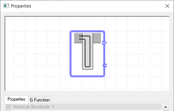
A vertical borehole is a type of ground source heat exchanger that can heat or cool the fluid going through it depending on the temperatures of the fluid and the ground.
The Vertical Borehole component in TAS comes with a G-function importer, which allows the user to import a pre-defined G – function, which will dictate the thermal response of the borehole.
Please note that the ground temperatures will depend on the results of the previous hours and the thermal properties entered for the ground in the Borehole’s properties.
Also in the results section, a positive load indicates the borehole is transferring heat out of the water to the ground while a negative load indicates the borehole is transferring heat from the ground to the water.
Controllers cannot be used with this component.
Properties
Name
This is the name of the component, it will be used in reports or error messages. You can rename components as you wish.
Description
The Description field allows the user to enter a description of the component. By default it is left blank.
Design Pressure Drop
This field allows the user to enter the pressure drop of the fluid through the component.
The drop in pressure is caused by resistance to the flow and the value entered will affect the amount of energy used by the pump on this circuit.
If the “Not Used” option is selected for this field, the user will be asked to enter in a Capacity for the fluid loop through this component.
Number of Boreholes
This field allows the user to enter how many boreholes they want the component to model.
These boreholes will be identical and use the same G-function. If you import a G-function, this field will change depending on the G-function you import.
Borehole Length
In this field the user must enter the length of the borehole from top to bottom.
Borehole Diameter
In this field the user must enter the diameter of the borehole.
Ground Thermal Conductivity
This field requires the user to enter the thermal conductivity of the ground surrounding the borehole.
If the soil type varies in the ground around the borehole, then please take a weighted average for the thermal conductivity.
Ground Heat Capacity
This field requires the user to enter the heat capacity of the ground surrounding the borehole.
If the soil type varies in the ground around the borehole, then please take a weighted average for the heat capacity.
Ground Density
This field requires the user to enter the density of the ground that the borehole is placed into.
If the soil type is different around the borehole then please take a weighted average for the density.
G-Function Reference Ratio
The user should enter here the ratio of borehole radius to borehole length.
This ratio should be entered into the software as the value \(x\), where the ratio is \(1:x\).
This ratio is used to adjust the g-values when the geometry of the borehole isn’t an exact match to the g-function
Pipe Inside Diameter
Enter the internal diameter of the pipes in the vertical borehole.
Pipe Outside Diameter
Enter here the external diameter of the pipes in the vertical borehole.
Pipe Thermal Conductivity
In this field, please enter the thermal conductivity of the pipes running through the vertical borehole.
Grout Thermal Conductivity
In this field, please enter the thermal conductivity of the grout in the vertical borehole.
Average Ground Temp
In this field, the user will need to specify the average ground temperature of the ground the borehole is in.
The user has two options when setting this, they can enter in the temperature as a value (useful for deep boreholes as the further down you go the warmer the ground gets) or they can set it to be the same as the ground water temperature.
This value is set in the simulation dialog box.
G – Function Importer
A G-function is a function which dictates the thermal response of a vertical borehole.
To enter the vertical boreholes G-function into the component, the user must go to the G-Function tab.
From here the user can create their own G-function for the borehole or import one from the G-Function database by pressing on the import button.
Slinky Coil
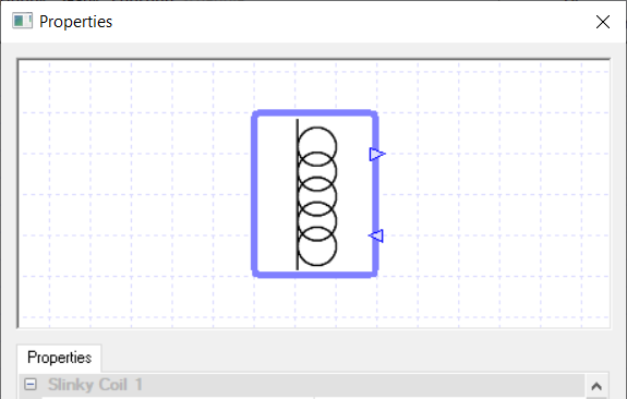
The Slinky Coil component in TAS systems allows the user to model vertical or horizontal slinky coils.
The slinky coil can provide heating or cooling depending on the temperature of the fluid going through it and the temperature of the ground.
Ground temperatures depend on: weather data, the thermal properties of the ground and the results of previous hours.
Please note that a negative load in the results section indicates heat transfer from the ground to the fluid while a positive load indicates heat transfer from the fluid to the ground.
Controllers cannot be used with this component.
Properties
Name
This is the name of the component, it will be used in reports or error messages. You can rename components as you wish.
Description
The Description field allows the user to enter a description of the component. By default it is left blank.
Design Pressure Drop
This field allows the user to enter the pressure drop of the fluid when passing through the component.
The drop in pressure is caused by resistance to the flow and the value entered will affect the amount of energy used by the pump on this circuit.
If the “Not Used” option is selected for this field, the user will be asked to enter in a Capacity for the fluid loop through this component.
Ground Density
This field requires the user to enter the density of the ground that the slinky coil is placed.
If the soil type is different around the slinky coil then please take a weighted average for the density.
Ground Specific Heat Capacity
This field requires the user to enter the specific heat capacity of the ground surrounding the slinky coil.
If the soil type varies in the ground around the slinky coil, then please take a weighted average for the specific heat capacity.
Ground Thermal Conductivity
This field requires the user to enter the thermal conductivity of the ground surrounding the slinky coil.
If the soil type varies in the ground around the slinky coil, then please take a weighted average for the thermal conductivity.
Ground Solar Reflectance
This field requires the user to enter in the solar reflectance of the top surface of the ground. It is used to calculate the heat gain of the soil from solar energy.
Pipe Inside Diameter
Enter the internal diameter of the pipes in the slinky coil.
Please note that this is for a cross section of pipe, not the diameter of a loop of pipe.
Pipe Outside Diameter
Enter here the external diameter of the pipes in the slinky coil.
Please note that this is for a cross section of pipe, not the diameter of a loop of pipe.
Pipe Thermal Conductivity
In this field, please enter the thermal conductivity of the pipes running through the slinky coil.
Trench Length
In this field, please enter the total length of the trench the slinky coil is sitting in.
Please note that this is the length of the trench and not the length of the pipes.
Trench Depth
In this field, please enter the depth of the trench.
The depth of the trench is the distance from the underside of the slinky coil to the top surface of the ground.
Loop Pitch / Displacement
The Loop Pitch / Displacement field requires the user to enter the interval between coil loops.
The interval the user should enter is shown in the diagram below as \(d\):
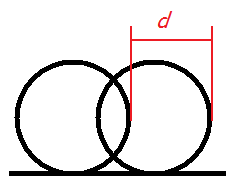
Coil Configuration
This field allows the user to set how the Slinky Coil is placed in the ground.
The user gets the following options to choose from:
Flat/horizontal
Upright/Vertical
Flat/horizontal
This option places the coils horizontally in the ditch.
Upon choosing this option the user is presented with the Loop Width field, where they should enter the diameter of the loops.
If the diameter of the slinky coil loops varies with each loop, then the user should enter the average here.
Upright/Vertical
This option places the coils vertically in the ditch.
Upon choosing this option the user is presented with the Loop Height field, where they should enter the diameter of the loops.
If the diameter of the slinky coil loops varies with each loop, then the user should enter the average here.
Surface Water Exchanger

The Surface Water Exchanger component is a water source heat exchanger which can be used to provide heating and cooling depending on the water temperatures.
The temperature of the body of water the exchanger is placed in depends on the results of previous hours, weather conditions and the geometry of the body of water.
Please note that the surface water exchanger component should not be used to model heat transfer with moving bodies of water (for example rivers) or for deep bodies of water (as it assumes perfect temperature mixing throughout the body of water). To emphasise this point the component will refer to the body of water as a pond in the properties.
Please note that controllers cannot be used with this component.
Properties
Name
This is the name of the component, it will be used in reports or error messages. You can rename components as you wish.
Description
The Description field allows the user to enter a description of the component. By default it is left blank.
Design Pressure Drop
This field allows the user to enter the pressure drop of the fluid when passing through the component.
The drop in pressure is caused by resistance to the flow and the value entered will affect the amount of energy used by the pump on this circuit.
If the “Not Used” option is selected for this field, the user will be asked to enter in a Capacity for the fluid loop through this component.
Efficiency
The Efficiency field allows the user to set the efficiency of the heat transfer between the body of water and the fluid circuit.
The efficiency is set by the following formula:
Where \(T_{return}\) is the temperature of the fluid leaving the surface water exchanger on the fluid circuit, \(T_{supply}\) is the temperature of the fluid entering the surface water exchanger on the fluid circuit and \(T_{mean}\) is the mean temperature of the body of water for the hour which can be found by taking the average of the current hours pond temperature and the previous hours pond temperature.
Pond Volume
In this field the user is required to enter the volume of the body of water.
Pond Surface Area
In this field the user is required to enter the surface area of the top surface of the pond (i.e. the surface that is not in contact with the ground).
Pond Perimeter
In this field the user is required to enter the perimeter of the body of water.
Ground Thermal Conductivity
This field requires the user to enter the thermal conductivity of the ground under and around the body of water.
If the soil type changes around the body of water then the user should take a weighted average for the thermal conductivity.
This field, along with the Pond Perimeter and Water Table Depth Beneath Pond field will be used to calculate heat transfer between the ground surrounding the body of water and the body of water.
Water Table Depth Beneath Pond
The user should enter here the depth of the water table beneath the pond.
To disregard the effects of ground heat transfer, the user should have a deep water table.
Horizontal Ground Heat Exchanger
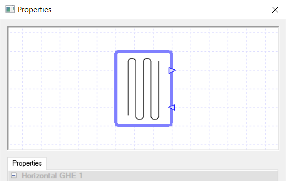
The Horizontal Ground Heat Exchanger (GHE) component in TAS systems allows the user to model a horizontal ground heat exchanger.
The Horizontal GHE is tailored to model a horizontal field of parallel pipes. This tailoring means that it cannot be used to model vertical pipes.
The Horizontal GHE can provide heating or cooling depending on the temperature of the fluid going through it and the temperature of the ground.
Normally a horizontal GHE would connect up to a heat pump, as it doesn’t have a setpoint to control the fluid temperatures.
In the simulation the ground temperatures depend on: weather data, the thermal properties of the ground and the results of previous hours.
Please note that a negative load in the results section indicates heat transfer from the ground to the fluid while a positive load indicates heat transfer from the fluid to the ground.
Controllers cannot be used with this component.
Properties
Name
This is the name of the component, it will be used in reports or error messages. You can rename components as you wish.
Description
The Description field allows the user to enter a description of the component. By default it is left blank.
Design Pressure Drop
This field allows the user to enter the pressure drop of the fluid through the component.
The drop in pressure is caused by resistance to the flow and the value entered will affect the amount of energy used by the pump on this circuit.
If the “Not Used” option is selected for this field, the user will be asked to enter in a Capacity for the fluid loop through this component.
Ground Density
This field requires the user to enter the density of the ground that the horizontal GHE is placed.
If the soil type changes around the horizontal GHE then please take a weighted average for the density.
Ground Specific Heat Capacity
This field requires the user to enter the specific heat capacity of the ground surrounding the horizontal GHE.
If the soil type varies in the ground around the GHE, then please take a weighted average for the specific heat capacity.
Ground Thermal Conductivity
This field requires the user to enter the thermal conductivity of the ground surrounding the horizontal GHE.
If the soil type varies in the ground around the GHE, then please take a weighted average for the thermal conductivity.
Ground Solar Reflectance
This field requires the user to enter in the solar reflectance of the top surface of the ground the horizontal GHE is placed in.
It is used to calculate the heat gain of the soil from solar energy.
Pipe Inside Diameter
Enter the internal diameter of the pipes in the horizontal GHE.
Please note that this is for a cross section of pipe.
Pipe Outside Diameter
Enter here the external diameter of the pipes in the horizontal GHE.
Please note that this is for a cross section of pipe.
Pipe Thermal Conductivity
In this field, please enter thermal conductivity of the pipes running through the Horizontal GHE.
Total Pipe Length
In this field the user should enter the total length of the pipe running through the GHE.
Pipe Separation
In this field, the user should enter the separation between the pipe as it snakes through the GHE.
If the separation between the pipe varies throughout the GHE, the user should take the average separation. This separation distance will have an effect on how effective the heat transfer is.
Please note that the maximum allowed separation is 2m.
Pipe Depth
In this field, please enter the depth of the pipe in the horizontal GHE.
The depth of the pipe is the distance from the underside of the pipe in the horizontal GHE to the top surface of the ground.
Boiler
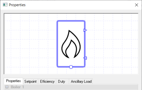
The Boiler component in TAS allows users to model boilers in their plant room circuits.
The boiler heats up the fluid passing through it to a setpoint by burning fuel. Please note that a boiler cannot provide any cooling.
Boilers are normally connected up to heating and DHW collections but can be used in other circuits.
Controllers
You can use a controller with the boiler to control it by informing it of the amount of power the boiler should use to heat up the fluid flowing through it.
The controller does this by sending a signal, between zero and one, to the boiler dictating the proportion of the boiler’s duty it should use to heat up the fluid.
So, for example, if the boiler received a signal of zero the boiler would not heat up the fluid flowing through it. While if it received a signal of 1 the boiler will heat up the fluid flowing through it using the maximum amount of power allowed from the Duty field.
If no controller is used, the sensor used to determine the fluid’s temperature for the Setpoint field is assumed to be directly after the return port of the boiler.
Properties
Name
This is the name of the component, it will be used in reports or error messages. You can rename components as you wish.
Description
The Description field allows the user to enter a description of the component. By default it is left blank.
Schedule
The Schedule field allows the user to apply a schedule to their component to detail the operational hours of the component.
If a schedule is applied by the user, then they should note that for all hours outside of the scheduled hours, the component will not operate.
In the case of the boiler, this will mean that the fluid will flow through the boiler unheated, even if there is a controller sending a non-zero signal to the boiler.
The default schedule option is always on, meaning that the component will operate 24/7.
Fuel Source
With this field the user can choose the fuel source of the boiler.
For the boiler, the fuel will be burned to produce the heat to warm the fluid up. The options provided in the drop-down menu for the fuel source come from the fuel sources placed in the fuel source folder.
If no fuel sources have been placed in this folder, the only option available will be the “none” option. If the “none” option is used, you will obtain a warning and the loads of the component will be discarded.
Ancillary Load Fuel Source
This option works in the same way as the Fuel Source option but allows the user to set the fuel source for the ancillary loads of the boiler.
Design Pressure Drop
This field allows the user to enter the pressure drop of the fluid when passing through the component.
The drop in pressure is caused by resistance to the flow and the value entered will affect the amount of energy used by the pump on the boiler’s circuit loop.
If the “Not Used” option is selected for this field, the user will be asked to enter in a Capacity for the fluid loop through this component.
Design Flow Delta T
The Design Flow Delta T field allows the user to size the flow rate of the circuit loop the component is on such that the fluid flowing through the component is kept within a certain temperature band.
The user can choose not to size the flow rate using this band, by choosing the “None” option.
If the user decides to use this option, by choosing the “Value” option, they will need to make sure that they have a pump on the same circuit loop as the component with the pump’s Design Flow Rate field set to “Sized”.
The value entered into the Design Flow Delta T field of the chiller affects the flow rate of the circuit loop in the following way. If the component has a setpoint of \(x\) and a Design Flow Delta T of \(y\), then the fluid will always be kept within the temperature range \(x-y\) to \(x+y\) when flowing through the component by ensuring the design flow rate of the circuit is sized high enough.
If multiple components / collections on the same circuit have a Design Flow Delta T value entered, TAS will take the results of the one which requires the highest design flow rate.
Please note that for components, the Design Flow Delta T will also size the flow rate so that the demand placed on the component is also met.
Setpoint
When a temperature is entered into the Setpoint field, the component will attempt to regulate the temperature of the fluid going through it to reach the setpoint.
In the case of the boiler, it will heat the fluid so it reaches the setpoint, but it will not be able to cool down the fluid to reach this setpoint. To cool the fluid you would need another component, for instance an air source chiller.
Please note that when a controller is used in conjunction with the boiler, the Setpoint field will disappear from the properties. This is done because the boiler is being controlled by a controller and will heat up the fluid when the controller sends a signal informing the boiler to do so.
When the Setpoint field is visible, modifiers can be added to the setpoint using the Setpoint tab.
Efficiency
Upon clicking on the Efficiency field, you will be transferred over to the Efficiency tab where you can create a profile for the efficiency using modifiers.
By default, a partload modifier is set up on the boiler efficiency so the user can enter the boilers efficiency at different part loads. If the user wishes, they can delete the modifier and enter in a value for the efficiency of the boiler. This is equivalent to having a partload modifier with the same efficiency entered at each step.
Duty
The duty of a component is the upper limit on the amount of power a component can provide.
If, in a certain hour, the power demand on the component is greater than the duty of the component, the component will not be able to meet this demand (For a boiler, it means it wouldn’t be able to heat up the fluid to the setpoint, it would fall short).
In TAS Systems, the demand met by a component is reported for each hour in the results section.
Currently, there are 3 options for setting the duty:
Unlimited
Sized
Value
In the duty tab, you will be able to choose these 3 options as well, but with the sized and value options you will be able to add a modifier.
Unlimited
Unlimited means the component is always able to meet the demand. Please note that this option cannot be used when a controller is attached to the component.
Sized
Allows the user to size the duty on a design condition. The user will also be asked for a size fraction and a method to size on. With the method option, you get to choose from the following options:
Add load, all attached – TAS Systems will size the duty of the component on the demand from all attached collections in the circuit.
Add load, local – TAS systems will size the duty of the component on the demand from all collections on the same loop as the component.
Add load, all attached heating - TAS will size the duty of the component on the demand from all heating collections in the circuit.
Add load, all attached DHW - TAS will size the duty of the component on the demand from all DHW collections in the circuit.
Please note that to size the duty the user will need to have design conditions in their systems file.
When using the “Sized” option the user also has the option to include or exclude storage losses from the sizing calculation. This is used to account for (or ignore) the additional load due to a Tank component in the same system.
Value
With this option the user will type in the duty of the component.
Ancillary Load
This field allows the user to model the load used by any additional ancillary services associated with the boiler.
Any value entered here will be the associated load during any hour the boiler operates, so it is advised to make use of the modifiers available with this field.
Examples of ancillary loads which might be associated with plantroom components include internal pumps and fans which are not accounted for in the consumption figure for the component.
Modifiers can be added to this field using the Ancillary Load tab.
Combined Heat and Power (CHP)
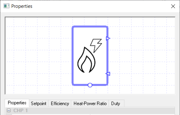
The CHP component in TAS systems allows users to model Combined Heat and Power (CHP) units.
As the TAS Systems wizard comes with a set up CHP circuit, it is recommended that the user uses the wizard when setting up CHP’s.
The user will notice in the Wizard a priority option which is not present in the properties list. The priority field in the wizard sets which loop (heating or DHW) the fluid out of the CHP reaches first.
CHPs normally cover the demand from heating and DHW collections but can also provide heat to absorption chillers.
Controllers
You can use a controller with the CHP to control it by informing it of the amount of power the CHP should use to operate.
The controller does this by sending a signal, between zero and one, to the CHP dictating the proportion of the CHP’s duty it should use to heat up the fluid and generate electricity.
So, for example, if the CHP received a signal of zero the CHP would not heat up the fluid flowing through it and not generate any electricity. While if it received a signal of 1 the CHP will heat up the fluid flowing through it and generate electricity using the maximum amount of power allowed from the Duty field.
If no controller is used, the sensor used to determine the fluid’s temperature for the Setpoint field is assumed to be directly after the return port of the CHP.
Properties
Name
This is the name of the component, it will be used in reports or error messages. You can rename components as you wish.
Description
The Description field allows the user to enter a description of the component. By default it is left blank.
Schedule
The Schedule field allows the user to apply a schedule to their component to detail the operational hours of the component.
If a schedule is applied by the user, then they should note that for all hours outside of the scheduled hours, the component will not operate.
In the case of the CHP, this will mean that the fluid flowing through the CHP will remain unheated and no power will be generated.
The default schedule option is always on, meaning that the component will operate 24/7.
Fuel Source
With this field the user can choose the fuel source of the CHP.
This fuel source will be the fuel the CHP unit burns to provide the heat and power. The options provided in the drop-down menu for the fuel source come from the fuel sources placed in the fuel source folder.
If no fuel sources have been placed in this folder, the only option available will be the “none” option. If the “none” option is used, you will obtain a warning and the loads of the component will be discarded.
Electrical Source
In this field the user should assign a “fuel source” to assign to the electricity produced from the CHP.
The reason for assigning a fuel source here is to set the tariff (for the cost report, normally the tariff would be negative for electricity you generate so the cost report will subtract it from the grid supplied electricity cost) and for the CO2 report (As generated electricity may have a different CO2 factor than electricity from the grid).
Normally the user would choose Grid Displaced Electricity for this field from the default fuel options from the library.
Design Pressure Drop
This field allows the user to enter the pressure drop of the fluid when passing through the component.
The drop in pressure is caused by resistance to the flow and the value entered will affect the amount of energy used by the pump on the CHP’s circuit loop.
If the “Not Used” option is selected for this field, the user will be asked to enter in a Capacity for the fluid loop through this component.
Design Flow Delta T
The Design Flow Delta T field allows the user to size the flow rate of the circuit loop the component is on such that the fluid flowing through the component is kept within a certain temperature band.
The user can choose not to size the flow rate using this band, by choosing the “None” option.
If the user decides to use this option by choosing the “Value” option, they will need to make sure that they have a pump on the same circuit loop as the component with the pump’s Design Flow Rate field set to “Sized”.
The value entered into the Design Flow Delta T field of the chiller affects the flow rate of the circuit loop in the following way. If the component has a setpoint of \(x\) and a Design Flow Delta T of \(y\), then the fluid will always be kept within the temperature range \(x-y\) to \(x+y\) when flowing through the component by ensuring the design flow rate of the circuit is sized high enough.
If multiple components / collections on the same circuit have a Design Flow Delta T value entered, TAS will take the results of the one which requires the highest design flow rate.
Please note that for components, the Design Flow Delta T will also size the flow rate so that the demand placed on the component is also met.
Setpoint
When a temperature is entered into the Setpoint field, the component will attempt to regulate the temperature of the fluid going through it to reach the setpoint.
In the case of the CHP, it will heat the fluid so it reaches the setpoint, but it will not be able to cool down the fluid to reach this setpoint. To cool the fluid you would need another component, for instance an air source chiller.
Please note that when a controller is used in conjunction with the CHP, the Setpoint field will disappear from the properties. This is done because the CHP is being controlled by a controller and will heat up the fluid when the controller sends a signal informing the CHP to do so.
When the Setpoint field is visible, modifiers can be added to the setpoint using the Setpoint tab.
Efficiency
Upon clicking on the Efficiency field, you will be transferred over to the Efficiency tab where you can create a profile for the efficiency using modifiers.
By default, a partload modifier is set up on the CHP efficiency so the user can enter the CHP’s efficiency at different part loads.
If the user wishes, they can delete the modifier and enter in a value for the efficiency of the CHP. This is equivalent to having a partload modifier with the same efficiency entered at partload.
The user should note that the efficiency entered for the CHP is the combined heat and power efficiency.
Heat to Power Ratio
This ratio is used to set the power generated by the CHP based on the heating demand.
The ratio used is heating demand: power generated and the value entered in this field is the heating demand side of the ratio when the power generated side is one (So if the ratio was 3:1, the user would enter a value of 3 in this field).
Please note that the user can add a modifier to this field using the Heat-Power Ratio tab.
Duty
The duty of a component is the upper limit on the amount of power a component can provide.
If, in a certain hour, the power demand on the component is greater than the duty of the component, the component will not be able to meet this demand (For a CHP, it means it wouldn’t be able to heat up the fluid to the setpoint, it would fall short).
In TAS Systems, the demand met by a component is reported for each hour in the results section.
Currently, there are 3 options for setting the duty:
Unlimited
Sized
Value
In the duty tab, you will be able to choose these 3 options as well, but with the sized and value options you will be able to add a modifier.
Unlimited
Unlimited means the component is always able to meet the demand. Please note that this option cannot be used when a controller is attached to the component.
Sized
Allows the user to size the duty on a design condition. The user will also be asked for a size fraction and a method to size on. With the method option, you get to choose from the following options:
Add load, all attached – TAS Systems will size the duty of the component on the demand from all attached collections in the circuit.
Add load, local – TAS systems will size the duty of the component on the demand from all collections on the same loop as the component.
Add load, all attached heating - TAS will size the duty of the component on the demand from all heating collections in the circuit.
Add load, all attached DHW - TAS will size the duty of the component on the demand from all DHW collections in the circuit.
Add load, all attached Chillers - TAS will size the duty of the component on the demand from all Chillers on the circuit. This option could be used with absorption chillers, allowing the CHP to provide the heat necessary to drive the absorption chiller’s cooling system.
Please note that to size the duty the user will need to have design conditions in their systems file.
When using the “Sized” option the user also has the option to include or exclude storage losses from the sizing calculation. This is used to account for (or ignore) the additional load due to a Tank component in the same system.
Value
With this option the user will type in the duty of the component.
Multi Boiler
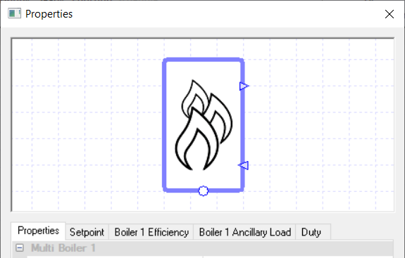
The Multi Boiler component allows the user to model multiple boilers using only one component.
Please note that any field beginning with “Boiler X …”, where X is a positive integer, is unique to the Xth boiler. The other fields (apart from: duty, sequence and multiplicity) are the same for each boiler.
Please note that the duty is the amount of demand all the boilers combined could meet, each boiler’s individual duty is set by the “boiler X percentage” field. So if the Multi Boiler is modelling 3 boilers, then each boiler will have the same setpoint while their fuel sources will be dependent on the field “Boiler X fuel source”.
Properties
As boilers have been discussed previously, only the new properties will be discussed.
Multiplicity
The number in the multiplicity field represents how many boilers the Multi boiler is representing.
Boiler X Percentage
This option allows the user to set the duty of the Xth boiler.
The user will enter a percentage in this field which will set the boilers duty as this percentage of the total duty in the duty field.
Please note that the sum of all the “Boiler X Percentage” fields must add up to 100%. Not doing so will give you a warning and incorrect results.
Sequence
The Sequence field tells the component how the multiple Boilers will be set up. The user has three options to choose from:
Parallel - The load is split up between the boilers. The load will be split evenly until one of the boilers reaches its duty.
Serial - The first boiler covers the load until it reaches its duty. At that point the second boiler would start to cover the load and so on.
Staged - With a staged setup only the first boiler runs at part load. As the first boiler normally has a bigger duty than the other chiller; once one of the other boilers can run at full load the load will transition to that boiler.
Solar Panel
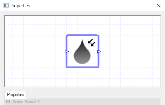
The Solar Panel component in TAS Systems allows the user to model solar hot water panels, which convert the solar energy absorbed by the panel to heat which warms up the fluid passing through the solar panel.
Please note that the user can choose whether to use a surface from their model or create a surface by specifying the values directly into the properties of the component.
Controllers cannot be used with this component.
Properties
Name
This is the name of the component, it will be used in reports or error messages. You can rename components as you wish.
Description
The Description field allows the user to enter a description of the component. By default it is left blank.
Design Pressure Drop
This field allows the user to enter the pressure drop of the fluid through the component.
The drop in pressure is caused by resistance to the flow and the value entered will affect the amount of energy used by the pump on the Solar Panel’s circuit loop.
If the “Not Used” option is selected for this field, the user will be asked to enter in a Capacity for the fluid loop through this component.
Maximum Panel Efficiency (“Eta -0”)
In this field the user will need to input the Eta- 0 value of their solar panel.
The Eta – 0 value can be obtained from the solar panel’s manufacturer and it details the efficiency of panel at transferring solar energy into heat.
1st order heat loss coefficient (Alpha – 1)
In this field the user will need to input the Alpha – 1 value of their solar panel.
The Alpha -1 value can be obtained from the solar panel’s manufacturer and it details the first order heat loss from the solar panel.
2nd order heat loss coefficient (Alpha – 2)
In this field the user will need to input the Alpha – 2 value of their solar panel.
The Alpha -2 value can be obtained from the solar panel’s manufacturer and it details the second order heat loss from the solar panel.
Multiplicity
The Multiplicity field allows the user to enter in a factor which is then multiplied by the surface area of the panel so that the component can model a smaller or larger array of panels.
This will be especially useful when using the component with a surface from a panel drawn in the 3D modeller, as this field allows you to modify the surface area of the panel from Systems rather than going back to the 3D modeller and making the changes there.
Calculation Method
This option allows the user to decide if they wish to calculate the dimensions of their solar panel using a surface from the TBD or if they wish to set the properties of the solar panel within TAS Systems.
If the user chooses to use the Use zone surface option they will need to drag a zone, which has a surface that has the solar panel box ticked, onto the component. TAS Systems will then use this surface to calculate the results.
The user can also choose the Specify Values option, where they will need to fill in the following information:
Area
Inclination
Orientation
Solar Reflectance
Please note that when using the “Specify Values” option, the solar gain on the panel due to solar energy being reflected from the surrounding ground is not included in the solar gain figures. To include this, the user will have to model the panel in the 3d modeller.
Area
Enter the area of the panel.
Inclination
Enter the angle the panel is tilted at in degrees: 0 degrees is facing upwards (horizontal panel), 90 degrees is a vertical panel, etc.
The user can also choose the “Sun tracking” option; with this option the panel will move its inclination to follow the sun’s path during the day.
Orientation
Here the user has two options. If they choose the “Value” option, the user is required to enter the orientation the panel is facing in degrees where: 0 degrees is north, 90 degrees is East etc.
The user can also choose the “Sun Tracking” option; with this option the panel will move its orientation to follow the sun’s path during the day.
Solar Reflectance
In this field the user should enter the solar reflectance of the panel’s surface as a factor between zero and one.
Design Flow Rate per m²
In this field the user enters the design flow rate of the fluid they require per \(\text{m}^2\) (per \(text{ft}^2\) in U.S Customary units).
If the pump on the circuit loop is set to sizing, it will set the design flow rate of the circuit loop by multiplying this field by the area of the panel.
Bypass if Generation is negative
Upon ticking this field, the fluid will bypass the solar panel in the hours where there is not enough solar energy to warm the fluid up to counter the heat loss it incurs by passing through the panel.
PV Panel
The PV panel component in TAS systems allows the user to model PV panels.
The PV panels do not connect up to any plant room circuit as they are only used to calculate the amount of electricity they will generate.
Please note that user can choose whether to use a surface from their model or create a surface by specifying the values directly into the properties of the component.
Controllers cannot be used with this component.
Properties
Name
This is the name of the component, it will be used in reports or error messages. You can rename components as you wish.
Description
The Description field allows the user to enter a description of the component. By default it is left blank.
Electrical Source
In this field the user should assign a “fuel source” which the electricity generated from the panel will be assigned to.
The reason for assigning a fuel source here is to set the tariff (for the cost report, normally the tariff would be negative for electricity you generate so the cost report will subtract it from the grid supplied electricity cost) and for the CO2 report (As generated electricity may have a different CO2 factor than electricity from the grid).
Normally the user would choose Grid Displaced Electricity for this field from the default options.
Efficiency Method
The method to use for calculating the panel efficiency. Can be:
Standard Test Conditions (STC): Enter the power output per unit are at Standard Test Conditions.
Detailed: User-specified solar conversion efficiency and inverter properties.
Solar Conversion Efficiency
This field is only shown when the “Detailed” Efficiency Method is used.
In this field the user should enter how efficient the PV panel is at converting the solar energy into electricity.
By default, a profile based on Irradiance has been set up in the Panel efficiency tab. The user can modify this profile, create a new one or delete the profile and just enter a value for the efficiency in per cent.
If a value is used, this efficiency is used for every hour of operation for the PV panel.
AC Inverter Size
This field is only shown when the “Detailed” Efficiency Method is used.
This field allows the user to set the size of the AC inverter. This sets the upper limit of how much electricity can be generated in one hour.
Multiplicity
The Multiplicity field allows the user to enter in a factor which is then multiplied by the surface area of the panel so that the component can model a smaller or larger array of panels.
This will be especially useful when using the component with a surface from a panel drawn in the 3D modeller, as this field allows you to modify the surface area of the panel from Systems rather than going back to the 3d modeller and making the changes there.
Inverter Efficiency
This field is only shown when the “Detailed” Efficiency Method is used.
The Inverter Efficiency field allows the user to input how efficient the inverter is at converting solar energy into electricity.
By default a partload profile modifier is set to this field detailing the inverter’s efficiency at different part loads. The user can edit or modify the modifiers or delete it and just enter a percentage value.
Output at STC
This field is only shown when the “Standard Test Conditions” Efficiency Method is used.
This is the electrical output per unit area at standard test conditions (1 kW/m2 of incident solar radiation on the panel).
Derating Factor
This field is only shown when the “Standard Test Conditions” Efficiency Method is used.
This is a factor reducing panel output based on shading, ventilation, etc.
For example a panel with 200W/m2 Output at STC and a Derating Factor of 0.9 would produce 180 W/m2 at standard test conditions.
Minimum Irradiance
This field set’s a minimum irradiance level that must be met for the PV panel to generate electricity.
If the irradiance in any hour is below this value, then no electricity will be generated.
Nominal Operating Cell Temperature
This field requires the user to enter the panel’s temperature when the efficiency was measured.
Power Temperature Coefficient
This field requires the user to enter the power temperature coefficient of the panel.
This is used to account for the decreased efficiency of the panel when it goes above the nominal operating cell temperature. To disregard the effect of panel temperature on efficiency, set this value to zero.
Calculation Method
This option allows the user to decide if they wish to calculate the dimensions of their PV panel using a surface from the TBD or to set the properties of the PV panel within systems.
If the user chooses to use the Use zone surface option, the user will need to drag a zone, which has a surface that has the PV panel box ticked, onto the component. TAS Systems will then use this surface to calculate the results.
The user can also choose the Specify Values option, where they will need to fill in the following information:
Area
Inclination
Orientation
Solar Reflectance
Please note that when using the Specify Values option, the solar gain on the panel due to solar energy being reflected from the surrounding ground is not included in the solar gain figures. To include this, the user will have to model the panel in the 3d modeller.
Area
Enter the area of the panel.
Inclination
Enter the angle the panel is tilted at in degrees: 0 degrees is facing upwards (horizontal panel), 90 degrees is a vertical panel, etc.
The user can also choose the “Sun tracking” option; with this option the panel will move its inclination to follow the sun’s path during the day.
Orientation
Here the user has two options. If they choose the “Value”, the user is required to enter the orientation the panel is facing in degrees where: 0 degrees is north, 90 degrees is East etc.
The user can also choose the “Sun tracking” option; with this option the panel will move its orientation to follow the sun’s path during the day.
Solar Reflectance
In this field the user should enter the solar reflectance of the panel’s surface as a factor between zero and one.
Wind Turbine
The Wind Turbine component in TAS systems allows the user to model vertical axis and horizontal axis wind turbines.
The wind turbine component does not connect up to any plant room circuits as they are only used to calculate the amount of electricity they will generate.
As the turbine is only used to generate electricity and do not link with any other component, controllers cannot be used with them.
Properties
Name
This is the name of the component, it will be used in reports or error messages. You can rename components as you wish.
Description
The Description field allows the user to enter a description of the component. By default it is left blank.
Electrical Source
In this field the user should assign a “fuel source” which the electricity generated from the turbine will be assigned to.
The reason for assigning a fuel source here is to set the tariff (for the cost report, normally the tariff would be negative for electricity you generate so the cost report will subtract it from the grid supplied electricity cost) and for the CO2 report (As generated electricity may have a different CO2 factor than electricity from the grid).
Normally the user would choose Grid Displaced Electricity for this field from the default options.
Hub Height
This field requires the user to enter the height of the turbine’s hub.
The height should be measured from the ground to the hub.
Please note that a higher hub will produce more electricity than a wind turbine with the same properties except from the hub being nearer the ground.
Swept Area
This field requires the user to enter the area the blades sweep out during a rotation. The bigger the area they sweep out, the more electricity the turbine produces.
For a vertical axis wind turbine the surface area is the side curved surface of the cylinder swept out by the blades.
Minimum Wind Speed
This field requires the user to enter the minimum wind speed required for the turbines to produce electricity.
Please note that if the wind speed is below this value for an hour then no electricity will be produced.
Cut – Off Wind Speed
This field requires the user to enter the maximum wind speed that the turbine will operate in.
If the wind speed goes above this cut off value in an hour, then the turbine will not produce any electricity in this hour.
Multiplicity
Allows the user to set how many wind turbines the component is modelling.
Please note that each wind turbine will have identical properties matching the values entered into the component.
Efficiency
The Efficiency field allows the user to input how efficient the wind turbine is at converting wind power into electricity.
By default a wind speed profile modifier is set to this field detailing the turbine’s efficiency at different wind speeds.
While the default modifier is based on wind speed, the user can edit to be based on a few different options, including wind direction. If they wish, the user can also delete the modifier and just enter a value into this field; this value will always be the efficiency of the wind turbine.
Heating Collection
A Heating Collection groups together a selection of heating coils / heating components that share a common source of heat.
To add an air-side component to a collection requires the user to select the collection in the heating collection field of the air-side component’s properties.
While sensors from a controller can be attached to the collection, a controller cannot be used to control any of the properties of a collection.
Properties
Name
This is the name of the component, it will be used in reports or error messages. You can rename components as you wish.
Description
The Description field allows the user to enter a description of the component. By default it is left blank.
Design Pressure Drop
This field allows the user to enter the design pressure drop of the fluid through the collection.
The drop in pressure is caused by resistance to the flow and the value entered will affect the amount of energy used by the pump on the collections circuit loop.
If the “Not Used” option is selected then the user will need to enter in the capacity of the collection.
Design Flow Delta T
The Design Flow Delta T field allows the user to size the flow rate of the circuit loop the component is on such that the fluid flowing through the component is kept within a certain temperature band.
The user can choose not to size the flow rate using this band, by choosing the None option.
If the user decides to use this option, by choosing the Value option, they will need to make sure that they have a pump on the same circuit loop as the component with the pump’s Design Flow Rate field set to Sized.
The value entered into the Design Flow Delta T field of the chiller affects the flow rate of the circuit loop in the following way. If the component has a setpoint of \(x\) and a Design Flow Delta T of \(y\), then the fluid will always be kept within the temperature range \(x-y\) to \(x+y\) when flowing through the component by ensuring the design flow rate of the circuit is sized high enough.
If multiple components / collections on the same circuit have a Design Flow Delta T value entered, TAS will take the results of the one which requires the highest design flow rate.
Please note that for components, the Design Flow Delta T will also size the flow rate so that the demand placed on the component is also met.
Variable Flow Capacity
The Variable Flow Capacity option allows the user to decide if the fluid loop the collection is on will have a variable flow or a constant flow.
If the user chooses “yes” the flow rate on the loop will vary while if the user chooses no then the flow rate will be constant.
Size Fraction
This property allows design flow rates associated with this collection to be oversized.
For example if a size fraction of 1.2 is entered, design flow rates will be oversized by 20% (see Design Flow Delta T above for more notes on flow sizing).
Minimum Return Temperature
The minimum return temperature sets a limit on the temperature of the fluid exiting the collection.
This field will not impact the flow rate of the circuit but if it is set to high with respect to the flow rate you will receive warnings informing you that the demand is greater than the supply.
An example of this field being set to high with respect to the flow rate can be easily seen when using the Design Flow Delta T field. Upon entering a Design Flow Delta T of \(y\) where the collection is being provided fluid at a temperature of \(x\) then the flow rate will be sized so that the fluid will always be kept within the temperature range \(x-y\) to \(x+y\) and also so that the demand is met. If the minimum return temperature is set in between this range, then any heat source will not be able to meet the demand of the collection due to the chosen flow rate and the limit on the return temperature.
If you do not wish to set a minimum return temperature then select the None option for this field.
Distribution Efficiency Method
The method to use for calculating the distribution efficiency. Can be:
Value: An unchanging factor applied to the load.
Profile: Use a profile to dynamically calculate the additional demand due to distribution.
Distribution Efficiency
This field requires the user to input how efficient the heating collection is at distributing the heat to the air-side components.
Please note that in the results section, the demand reported by the heating collection is always the total demand from all the components in the collection summed together.
The demand with the effects of the Distribution Efficiency included can be seen at boilers / CHP units on your circuit.
Distribution Heat Loss:
The fluid heat loss which increases the load on the collection, and which can have profile modifiers applied so that the heat loss result can be calculated dynamically on the basis of e.g. flow rate and fluid temperature.
Components Tab
This tab allows the user to view all of the components that are part of this collection. The user can reorder this list if they wish, please note that this will have no impact on the results.
Cooling Collection
A Cooling Collection groups together a selection of cooling coils / cooling components that share a common energy source.
To add an air-side component to a collection requires the user to select the collection in the cooling collection field of the air-side component’s properties.
While sensors from a controller can be attached to the collection, a controller cannot be used to control any of the properties of a collection.
Properties
Name
This is the name of the component, it will be used in reports or error messages. You can rename components as you wish.
Description
The Description field allows the user to enter a description of the component. By default it is left blank.
Design Pressure Drop
This field allows the user to enter the pressure drop of the fluid through the collection.
The drop in pressure is caused by resistance to the flow and the value entered will affect the amount of energy used by the pump on the collections circuit loop.
If the “Not Used” option is selected then the user will need to enter in the capacity of the collection.
Design Flow Delta T
The Design Flow Delta T field allows the user to size the flow rate of the circuit loop the component is on such that the fluid flowing through the component is kept within a certain temperature band.
The user can choose not to size the flow rate using this band, by choosing the None option.
If the user decides to use this option, by choosing the Value option, they will need to make sure that they have a pump on the same circuit loop as the component with the pump’s Design Flow Rate field set to Sized.
The value entered into the Design Flow Delta T field of the chiller affects the flow rate of the circuit loop in the following way. If the component has a setpoint of \(x\) and a Design Flow Delta T of \(y\), then the fluid will always be kept within the temperature range \(x-y\) to \(x+y\) when flowing through the component by ensuring the design flow rate of the circuit is sized high enough.
If multiple components / collections on the same circuit have a Design Flow Delta T value entered, TAS will take the results of the one which requires the highest design flow rate.
Please note that for components, the Design Flow Delta T will also size the flow rate so that the demand placed on the component is also met.
Variable Flow Capacity
The Variable Flow Capacity option allows the user to decide if the fluid loop the collection is on will have a variable flow or a constant flow.
If the user chooses Yes the flow rate on the loop will vary while if the user chooses No then the flow rate will be constant.
Size Fraction
This property allows design flow rates associated with this collection to be oversized.
For example if a size fraction of 1.2 is entered, design flow rates will be oversized by 20% (see Design Flow Delta T above for more notes on flow sizing).
Maximum Return Temperature
The maximum return temperature sets an upper limit on the temperature of the fluid exiting the collection.
This field will not impact the flow rate of the circuit but if it is set to low with respect to the flow rate you will receive warnings informing you that the demand is greater than the supply.
An example of this field being set to low with respect to the flow rate can be easily seen when using the Design Flow Delta T field. Upon entering a Design Flow Delta T of \(y\) where the collection is being provided fluid at a temperature of \(x\) then the flow rate will be sized so that the fluid will always be kept within the temperature range \(x-y\) to \(x+y\) and also so that the demand is met. If the maximum return temperature is set in between this range, then any chiller may not be able to meet the demand of the collection due to the chosen flow rate and the limit on the return temperature.
If you do not wish to set a minimum return temperature then select the None option for this field.
Distribution Efficiency Method
The method to use for calculating the distribution efficiency. Can be:
Value: An unchanging factor applied to the load.
Profile: Use a profile to dynamically calculate the additional demand due to distribution.
Distribution Efficiency
This field requires the user to input how efficient the cooling collection is at distributing the cooled fluid to the air-side components.
Please note that in the results section, the demand reported by the cooling collection is always the total demand from all the components in the collection summed together.
The demand with the effects of the distribution efficiency included can be seen at chillers on your circuit.
Distribution Heat Gain:
The fluid heat gain which increases the load on the collection, and which can have profile modifiers applied so that the heat loss result can be calculated dynamically on the basis of e.g. flow rate and fluid temperature.
Components Tab
This tab allows the user to view all of the components that are part of this collection.
The user can reorder this list if they wish, please note that this will have no impact on the results.
DHW Collection
A DHW Collection groups together a selection of zones that share a common source for their DHW.
To add a zone component to a collection requires the user to select the collection in the DHW collection field of the zones component’s properties.
While sensors from a controller can be attached to the collection, a controller cannot be used to control any of the properties of a collection.
Properties
Name
This is the name of the component, it will be used in reports or error messages. You can rename components as you wish.
Description
The Description field allows the user to enter a description of the component. By default it is left blank.
Design Pressure Drop
This field allows the user to enter the pressure drop of the fluid through the collection.
The drop in pressure is caused by resistance to the flow and the value entered will affect the amount of energy used by the pump on the collections circuit loop.
If the “Not Used” option is selected then the user will need to enter in the capacity of the collection.
Design Flow Delta T
The Design Flow Delta T field allows the user to size the flow rate of the circuit loop the component is on such that the fluid flowing through the component is kept within a certain temperature band.
The user can choose not to size the flow rate using this band, by choosing the None option. If the user decides to use this option, by choosing the Value option, they will need to make sure that they have a pump on the same circuit loop as the component with the pump’s Design Flow Rate field set to Sized.
The value entered into the Design Flow Delta T field of the chiller affects the flow rate of the circuit loop in the following way. If the component has a setpoint of \(x\) and a Design Flow Delta T of \(y\), then the fluid will always be kept within the temperature range \(x-y\) to \(x+y\) when flowing through the component by ensuring the design flow rate of the circuit is sized high enough.
If multiple components / collections on the same circuit have a Design Flow Delta T value entered, TAS will take the results of the one which requires the highest design flow rate.
Please note that for components, the Design Flow Delta T will also size the flow rate so that the demand placed on the component is also met.
Load Distribution
The Load Distribution field allows the user to decide how their DHW demand will be spread out throughout the day.
The DHW demand is set in the internal condition for each zone and this field allows the user to decide how TAS Systems distributes it, using the following three options:
Normal
Daily
Even
Normal
For each zone TAS will split the DHW demand up evenly over the hours that zone is occupied (TAS decides if a zone is occupied by looking at the occupancy gains field from the zones internal condition.).
Once the DHW demand is worked out for each hour for the zone, the DHW collection sums the hourly DHW for each zone to produce the hourly DHW demand for the collection.
Daily
TAS will work out the total DHW demand for the collection for each day by summing the DHW demand for each zone in the collection.
TAS will then distribute it evenly over any hour where a zone in the DHW collection is occupied.
Even
TAS will work out the total DHW demand for the collection for the whole year by summing the DHW demand for each zone in the collection.
TAS will then distribute it evenly over any hour where a zone in the DHW collection is occupied.
Minimum Return Temperature
The minimum return temperature sets a limit on the temperature of the fluid exiting the collection.
This field will not impact the flow rate of the circuit but if it is set to high with respect to the flow rate you will receive warnings informing you that the demand is greater than the supply.
An example of this field being set to high with respect to the flow rate can be easily seen when using the Design Flow delta T field. Upon entering a Design Flow Delta T of \(y\) where the collection is being provided fluid at a temperature of \(x\) then the flow rate will be sized so that the fluid will always be kept within the temperature range \(x-y\) to \(x+y\) and also so that the demand is met.
If the minimum return temperature is set in between this range, then any heat source will not be able to meet the demand of the collection due to the chosen flow rate and the limit on the return temperature.
If you do not wish to set a minimum return temperature then select the “None” option for this field.
Distribution Efficiency Method
The method to use for calculating the distribution efficiency. Can be:
Value: An unchanging factor applied to the load.
Profile: Use a profile to dynamically calculate the additional demand due to distribution.
Distribution Efficiency
This field requires the user to input how efficient the DHW collection is at distributing the hot water to the zones.
Please note that in the results section, the demand reported by the DHW collection is always the total demand from all the zones in the collection summed together.
The demand with the effects of the distribution efficiency included can be seen at boilers / CHP units on your circuit.
Distribution Heat Loss:
The fluid heat loss which increases the load on the collection, and which can have profile modifiers applied so that the heat loss result can be calculated dynamically on the basis of e.g. flow rate and fluid temperature.
Components Tab
This tab allows the user to view all of the components that are part of this collection. The user can reorder this list if they wish, please note that this will have no impact on the results.
Refrigerant Collection
A Refrigerant Collection groups together a selection of refrigerant coils that share a common energy source.
Please note that in the plant room, Refrigerant Collections can only be attached to refrigerant components, like for example heat pumps.
The refrigerant only connections are highlighted by the collection having light blue ports on its side, to indicate that only refrigerant components can be connected to it.
To add an air-side component to a collection requires the user to select the collection in the Refrigerant Collection field of the air-sides component’s properties.
While sensors from a controller can be attached to the collection, a controller cannot be used to control any of the properties of a collection.
Properties
Name
This is the name of the component, it will be used in reports or error messages. You can rename components as you wish.
Description
The Description field allows the user to enter a description of the component. By default it is left blank.
Pipe Length
The Pipe Length field allows the user to enter in the length of the refrigerant pipes that run through the refrigerant collection.
While this field is not used directly by the calculations it can be used by modifiers on the heat pump, for instance when the user imports a Mitsubishi heat pump into their file the capacities will have a pipe length modifier applied to them.
Components Tab
This tab allows the user to view all of the components that are part of this collection. The user can reorder this list if they wish, please note that this will have no impact on the results.
Fuel Collection
A Fuel Collection can be used instead of a heating collection to group together a selection of heating coils / heating components that directly burn fuel at the air-side component to produce heat, instead of being connected up to boilers and other plant room components.
As the fuel collection is used to model the fuel being used at the air-side component, it does not have any ducts to connect up to plant room components.
To add an air-side component to a fuel collection requires the user to select the collection in the heating collection field of the air-sides component’s properties.
While sensors from a controller can be attached to the collection, a controller cannot be used to control any of the properties of a collection.
Properties
Name
This is the name of the component, it will be used in reports or error messages. You can rename components as you wish.
Description
The Description field allows the user to enter a description of the component. By default it is left blank.
Fuel Source
With this field the user can choose the fuel source of the fuel collection.
For the fuel collection, the fuel selected here will be burned to produce the heat at each coil / component which is a member of this collection.
The options provided in the drop-down menu for the fuel source come from the fuel sources placed in the fuel source folder. If no fuel sources have been placed in this folder, the only option available will be the “none” option.
If the “none” option is used, you will obtain a warning and the loads of the component will be discarded.
Components Tab
This tab allows the user to view all of the components that are part of this collection. The user can reorder this list if they wish, please note that this will have no impact on the results.
Electrical Collection
The main use of an Electrical collection is to group together electrical demands from lighting and equipment for reporting purposes, although it can be used instead of a heating collection to group together a selection of heating coils / heating components that generate heat using electricity as a fuel source.
As the electrical collection is used to model electricity being used by the components directly in the air-side systems, it does not connect up to any plant room components.
To add an air-side component to an electrical collection requires the user to select the collection in the heating collection or electrical collection field of the air-sides component’s properties.
While sensors from a controller can be attached to the collection, a controller cannot be used to control any of the properties of a collection.
Properties
Name
This is the name of the component, it will be used in reports or error messages. You can rename components as you wish.
Description
The Description field allows the user to enter a description of the component. By default it is left blank.
Electrical Source
With this field the user can choose the Electrical source of the electrical collection.
The electrical source chosen here will be the electricity provided to the members of this group. The options provided in the drop-down menu come from the fuel sources placed in the fuel source folder, so the user will be able to choose a non-electrical fuel source but this is not advised.
If no fuel sources have been placed in this folder, the only option available will be the “none” option.
If the “none” option is used, you will obtain a warning and the loads of the component will be discarded.
Components Tab
This tab allows the user to view all of the components that are part of this collection. The user can reorder this list if they wish, please note that this will have no impact on the results.