Internal Conditions
In the Building Simulator, Internal Conditions are applied to zones in order to describe the internal gains a zone will experience during a dynamic simulation.
Each internal condition applies on certain Day Types.
Warning
Each zone can only have a single internal condition per day type; in other words, it must not have multiple Internal Conditions that apply to the same day types.
Each Internal Condition can be assigned to multiple zones, and the Internal Conditions you select for a space will depend on the type of analysis you are performing in the Building Simulator.
Which Internal Conditions should I use?
For most types of overheating analysis and for calibrated energy models, you should create internal conditions that most closely reflect the real world internal gains the zone you are modelling will experience.
For UK Building regulations, you must use the National Calculation Methodology (NCM) internal conditions from the corresponding NCM Internal Conditions database; these must not be modified. For more information, see the UK Building Regulations Utility manual.
Creating Internal Conditions
Internal Conditions can be created in the Internal Conditions database via the New IC tab in the ribbon.
You can transfer Internal Conditions from the database to your Building Simulator file by dragging and dropping them onto the tree-view in the Building Simulator:
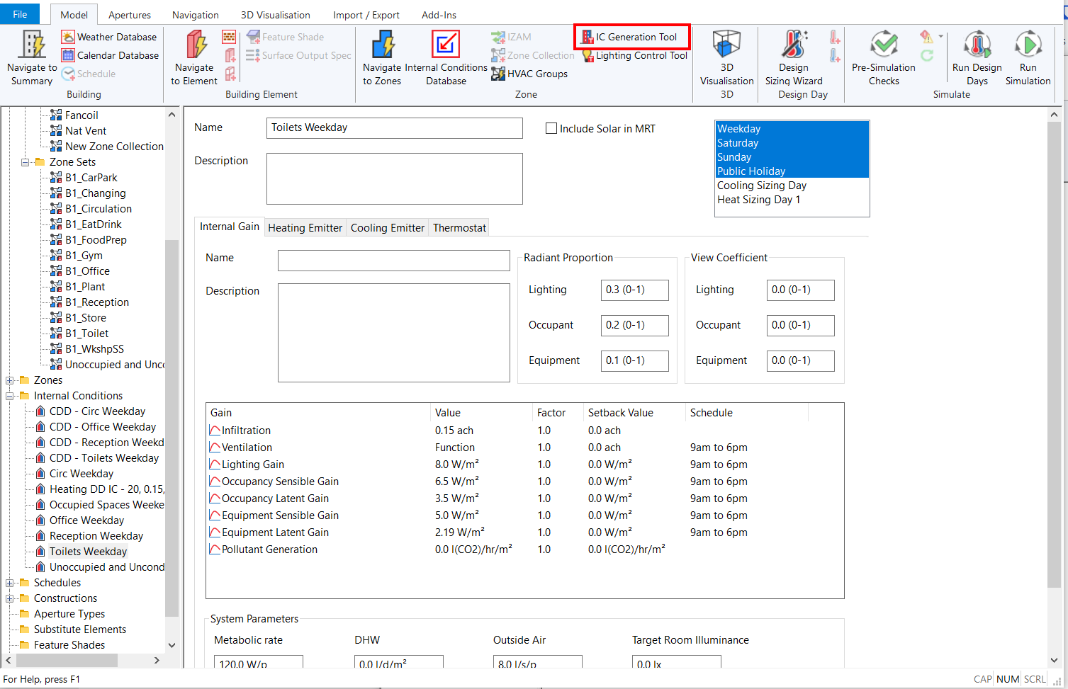
You can also create internal conditions using the IC Generation Tool, which can be launched from the ribbon:
You can remove internal conditions from a Building Simulator file by right clicking on the Internal Condition in the Internal Conditions list and pressing the Delete key on the keyboard.
Tip
You can find out which Internal Conditions aren’t assigned to any zones via the Pre Simulation Checks.
Assigning To Zones
You can assign Internal Conditions to Zones by dragging and dropping them from the internal conditions folder in the tree-view onto the zone in either the zones list or in the tree-view:
You can also drag and drop Internal Conditions from the tree-view onto the Internal Conditions tab of a zone:
You can remove internal conditions from a zone by selecting the Internal Condition in the Internal Conditions tab of the Zone and pressing the Delete key on the keyboard.
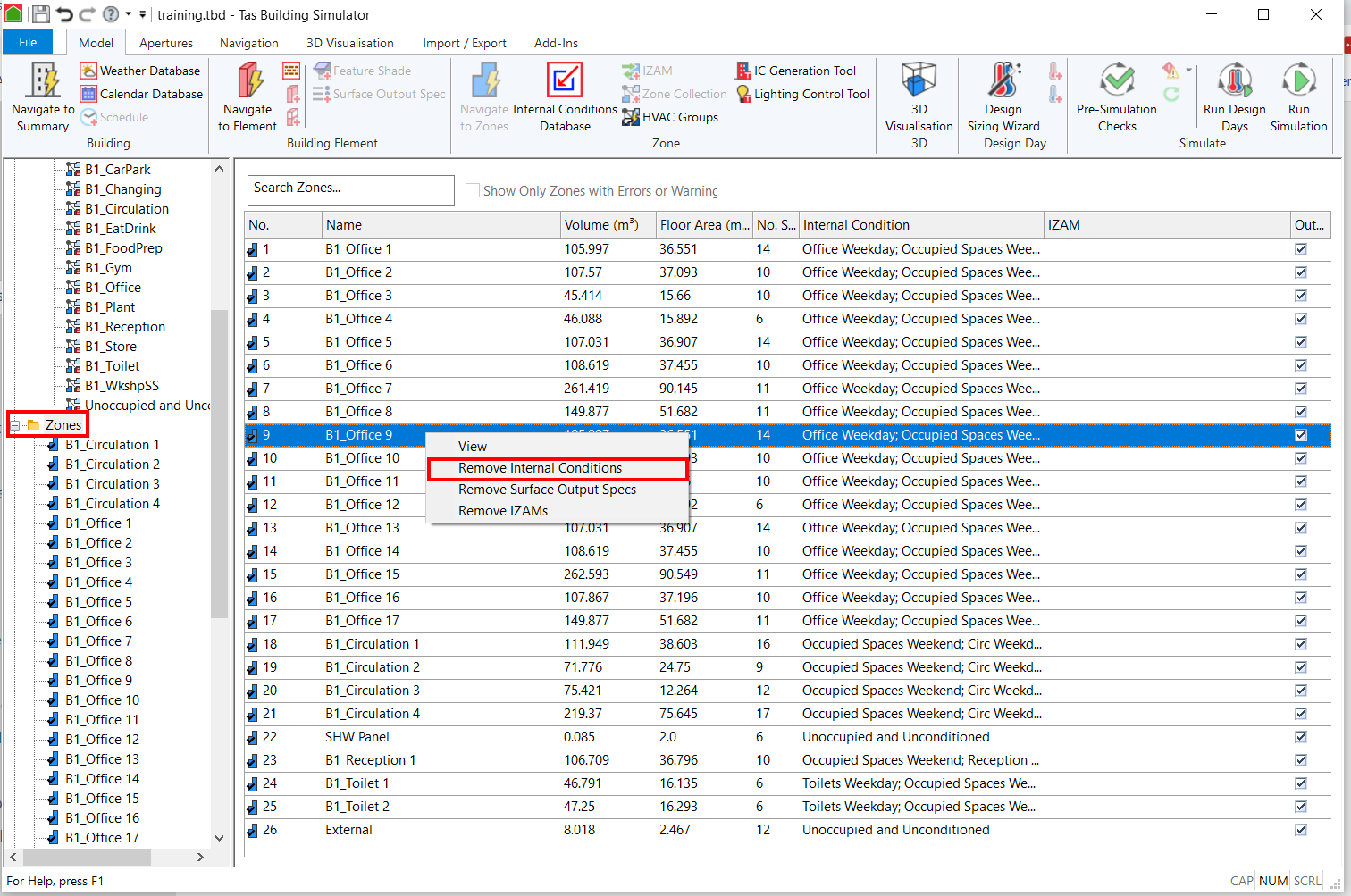
You can remove all Internal Conditions from a zone by right clicking on the zone in the zones list and selecting Remove Internal Conditions:
If you create Internal Conditions using the IC Generation Tool, they will automatically be assigned to zones.
Assigning Day Types
Day types can be assigned to an Internal Condition by left clicking on them in the list in the Internal Condition:
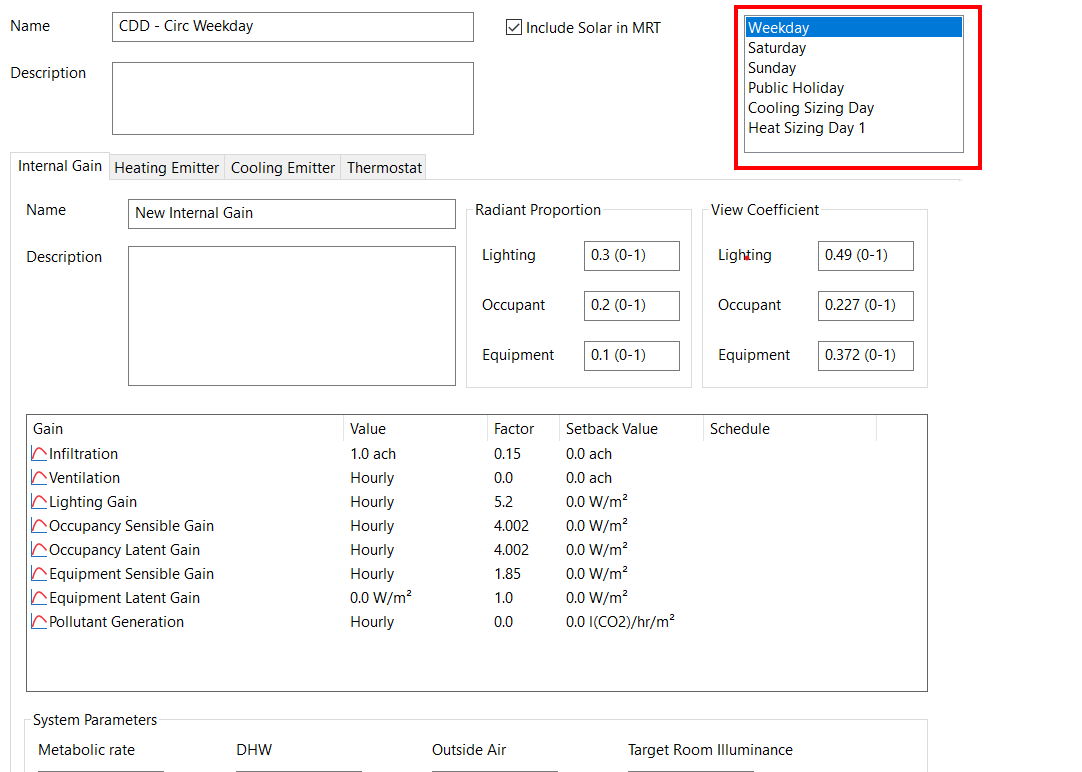
Each Internal Condition can be assigned to multiple day types. When the day type is highlighted, it is applied to that day type.
Include Solar in MRT
As part of the dynamic simulation, Tas calculates the Mean Radiant Temperature (MRT) of a zone for each hour of the year.
This checkbox determines whether or not Tas will take the diffuse solar radiation flux, which an occupant of a zone would experience, into account when calculating the MRT.
Including solar in MRT produces the most accurate estimate of the perceived mean radiant temperature.
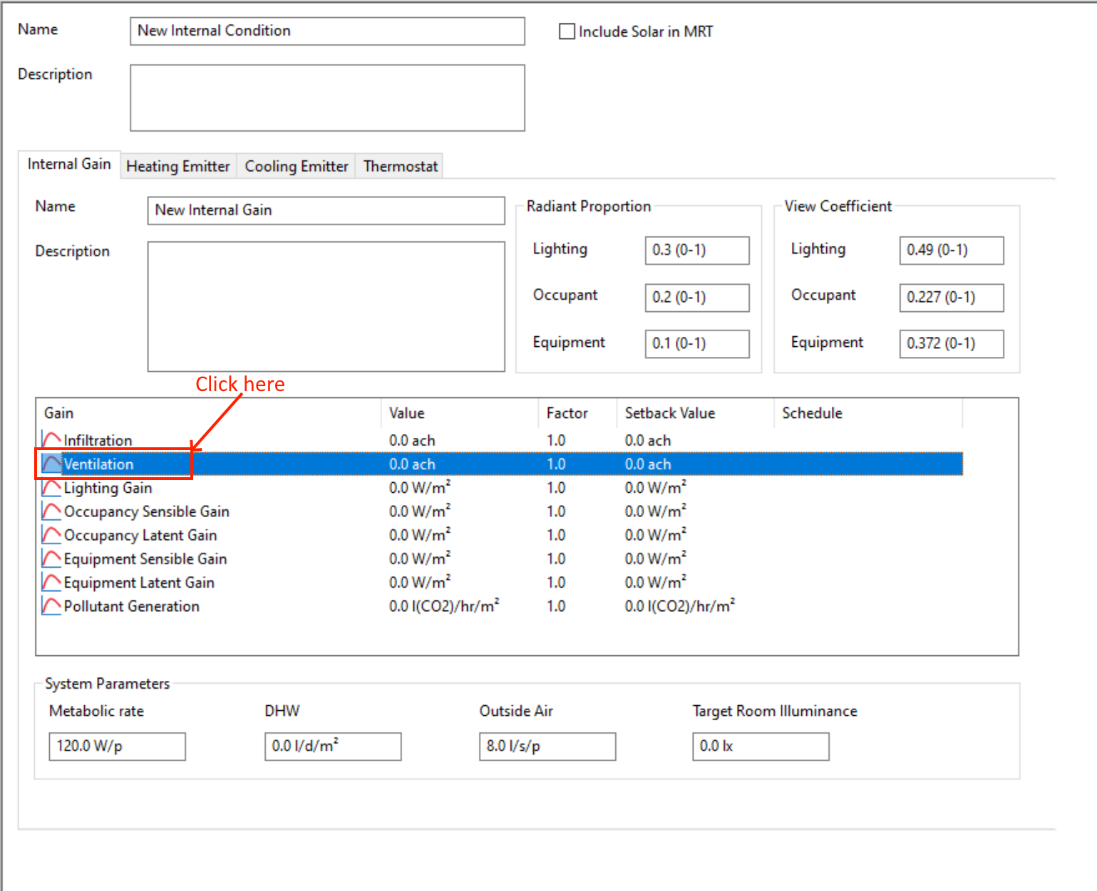
Internal Gains
The Internal Gains tab of an Internal Condition describes the following sources of thermal energy being added and removed from a space:
Heat gain/loss from Infiltration, ventilation
Heat from lighting
Heat gain from occupants
Heat gain from equipment
This tab also allows you to model sources of pollutant in the space such as Carbon Dioxide from occupants.
For each of the thermal gains in this tab, you can specify how much of that energy is transferred to the space via convection and via radiation (radiant proportion), and how much of the heat source is directly exposed to the occupants for radiative heat transfer (view coefficient).
Infiltration
Measured in Air Changes per Hour (ACH), this field represents the amount of air leakage into the zone.
The infiltration can be influenced by setting an infiltration coefficient in the Heating Plantroom Controls.
Ventilation
This field represents the amoutn of fresh air which enters the zone via mechanical ventilation.
Measured in Air Changes per Hour (ACH), this parameter makes it possible for you to obtain an estimate of the total load on an air handling system serving the building prior to detailed analysis in Tas Systems.
In addition to specifying the ventilation rates for every hour of the year, there are also a number of ventilation functions in the Building Simulator that model dynamic ventilation rates - such as ventilation rates that vary based on a zones dry bulb temperature. For more information, see Ventilation Functions.
Lighting Gain
Measured in Watts per Meter Squared (\(W/m^2\)), this field represents the amount of heat energy entering the space due to artificial lighting.
This gain has a number of functions which can be used to alter the lighting gain depending on the lux level in the space, for example, to model photocell control dimming.
For more information, see Lighting Control Functions.
Occupancy Sensible Gain
This field models the sensible heat transferred to a zone as a result of the metabolism of the occupants.
The amount of gain per occupant will therefore depend on the age of the occupant and their level of activity.
For an adult in an office environment, \(75W/m^2\) per person is a realistic figure - see CIBSE guide A for more information.
Occupancy Latent Gain
This field models the latent heat transferred to a zone as a result of the metabolism of the occupants - specifically, the fact that they add moisture to the space by exhalation.
The amount of gain per occupant will therefore depend on the age of the occupant and their level of activity.
For an adult in an office environment, \(55W/m^2\) per person is a realistic figure - see CIBSE guide A for more information.
Equipment Sensible Gain
This field represents the sensible heat gain to a zone as a result of equipment. This field has units of Watts per floor area.
Equipment Latent Gain
This field represents the sensible heat gain to a zone as a result of equipment adding moisture to the air. This field has units of Watts per floor area.
Pollutant Generation
The pollutant field can be used to represent any kind of pollutant, which has a default concentration of 350ppm (see the Building Summary). This can be a single value, a hourly profile or a yearly profile.
The pollutant in the building summary can, in addition, enter the space via infiltration and mechanical ventilation.
Radiant Proportion
The Radiant Proportion represents the proportion of an emitter which is in the form of radiant energy. Typical values are given below.
Emitter Category |
Emitter Type |
Radiant Proportion |
Heating |
Warm Air Heaters, Air Conditioning
Convectors
Natural
Radiator Type
Radiators
Multi-Column
Double and Treble
Double Column
Single Column
Floor Warming Systems
Block Storage Heaters
Panel Heaters
Wall
Ceiling
High Temperature Radiant Systems
|
0.00
0.10
0.10
0.20
0.30
0.30
0.50
0.50
0.15
0.67
0.67
0.90
|
Cooling |
Air Conditioning
Panel Coolers
Wall
Ceiling
Chilled Beams
|
0.00
0.58
0.58
0.15
|
Lights |
Tungsten
Fluorescent
|
0.80
0.48
|
Occupants |
0.20 |
|
Equipment |
0.10 |
View Coefficient
The View Coefficient fields are used by the software when calculating the mean radiant and resultant (operative) temperature in Tas. This field describes the degree to which radiation from the emitter contributes to the occupants’ perception of the radiant environment.
For most purposes, the values of view coefficients may be taken from the last column of the following table.
The table indicates the formula applicable to each type of emitter, and suitable values for the correction factors appearing in that formula. The values in the last column have been calculated for a room of dimensions 5m x 5m, and in the cases dealing with ceiling and floor heating, the value of e (distance between observer and emitting plane) is taken to be 1.3m.
Conditions under which these values may not be valid include the following:
Large rooms (dimensions much greater than 5m).
Ceiling emitters or other overhead emitters where the value of e is significantly different from 1.3m.
In such cases the formulae should be used (see below).
When applying the formulae, it should be understood that the dimensions referred to are those of a typical room, not those of the Tas zone.
If the room contains emitters of different types within a given emitter category, (for example, ceiling lighting and task lighting), the view coefficient can be calculated as an average of the view coefficients appropriate to each emitter, weighted in proportion to emitter power.
For Lambertian emitters, (which in practice, means all emitters except high temperature radiant heaters where the radiation is beamed using reflectors), the view coefficient \(C\) is defined as:
Equation 6.4-0
From this definition, it can be shown that the contribution of the emitter to the irradiance (\(W/m^2\)) at the observer position is:
Where \(W\) is the radiant power of the emitter per unit floor area. This relation is used in the calculation of the emitters contribution to mean radiant temperature.
As a guide to the effect of the view coefficient in mean radiant temperature calculations, the following relation, giving an approximation to the elevation of mean radiant temperature (in °C) due to a radiant heat source may be used:
Where \(W\) is the radiant component of the source in Watts/(m2 floor area).
Thus, a lighting gain of \(20W/m^2\) with a radiant proportion of \(0.48\) and a view coefficient of \(0.457\) causes an elevation in perceived mean radiant temperature of approximately:
The accurate calculation of a view coefficient for different emitter types and room geometries is complicated and involves numerical integration. However approximate formulae have been derived covering a range of situations and these are set out below.
Ceiling/Floor Emitters
This covers emitters distributed over a plane above the observer’s head (e.g. ceiling panel heaters, chilled beams, ceiling lights) and floor heating systems. We assume the room is rectangular. For this case, the formula for \(C\) is:
\(F_s\) = correction factor for emitter spectrum (lights only) = \((\frac{\alpha}{\epsilon})p_s + 1 - p_s\). Here, \(p_s\) is the proportion of emitter radiant output which is in the short-wave part of the spectrum. \(\frac{\alpha}{\epsilon}\) is the ratio of short wave absorptance to emissivity for skin. Taking \(\alpha\) = 0.8 for the lights spectrum and \(\epsilon\) = 0.98 this gives, for two common types of light:
Type of Light |
\(p_s\) |
\(F_s\) |
Tungsten |
0.111 |
0.980 |
Fluorescent |
0.313 |
0.948 |
The factor of 0.9 in the expression for \(C\) allows for a statistical distribution of observers (occupants) over the room. Without this factor, the expression applies to an observer in the centre of the room.
Overhead Radiant Heaters
Overhead radiant heaters direct the radiation downward in a narrow beam. Consequently an array of ceiling-mounted radiant heaters produces a radiation field similar to that experienced from non-beamed ceiling heaters in a room of large dimensions. Under these conditions equation 6.4-1 simplifies to:
Equation 6.4-2
Wall Emitters
This covers emitters set into the walls of the room (e.g.. radiators, wall panel heaters, wall-mounted lights).
For this case, the formula for \(C\) is:
Equation 6.4-3
The formula for \(C\): is an approximation based on numerical analysis of a range of cases. The calculations were done on the basis of a statistical distribution of observers over a region of the floor plan which excludes a 1m strip around the perimeter. The emitters were assumed to be distributed over a panel attached to one wall of the room and having a height of 1m; the results are similar when the emitters are distributed over two adjacent walls or when the panel height is varied by up to a factor of 2.
Distributed Emitters
This covers emitters distributed over the room such as computers or task lighting. The emitters are assumed to be distributed over a plane at the same height as the observer.
For this case, the formula for \(C\) is:
Equation 6.4-4
The formula for \(C\) is an approximation based on numerical analysis of a range of cases. The calculations were done on the basis of a statistical distribution of emitters over the entire floor plan and a statistical distribution of observers over a region of the floor plan which excludes a 1m strip around the perimeter. The calculations further assumed that no emitter is closer than 1m to an observer. The emitters were assumed to be distributed over a panel attached to one wall of the room and having a height of 1m; the results are similar when the emitters are distributed over two adjacent walls or when the panel height is varied by up to a factor of 2.
Heating Emitter
This tab allows you to change the Radiant Proportion and View Coefficient of the Heating Emitter.
You can also specify the external temperature range the plant can operate within.
Outside Temperature - Max - Below this external temperature, heating is available at its maximum capacity.
Outside Temperature - Off - Above this temperature, the heating is unavailable.
When the external temperature is between these two values, the plant capacity is proportionally varied.
Capacity Compensation
Enabling the Capacity Compensation for the Heating Emitter allows you to adjust the capacity of the heating based on the heating load the zone is currently experiencing.
The Heating Factor is a proportion of the zone’s maximum heating load.
Cooling Emitter
This tab allows you to change the Radiant Proportion and View Coefficient of the Cooling Emitter.
You can also specify the external temperature range the plant can operate within.
Outside Temperature - Max - Above this external temperature, cooling is available at its maximum capacity.
Outside Temperature - Off - The outside air temperature at and below which the cooling is switched off.
When the external temperature is between these two values, the plant capacity is proportionally varied.
Capacity Compensation
Enabling the Capacity Compensation for the Cooling Emitter allows you to adjust the capacity of the cooling based on the cooling load the zone is currently experiencing.
The Cooling Factor is a proportion of the zone’s maximum cooling load.
Thermostat
The options on the Thermostat tab allow you to control the set points for the heating, cooling and humidity of the zones the Internal Condition is applied to.
The Upper Limit relates to cooling. To model no cooling, you should set the Upper Limit to 150°C - this means cooling will only be required if the zones temperature exceeds 150°C, which should never happen.
The Lower Limit relates to heating. To model no heating, you should set the Lower Limit to -50°C - this means heating will only be required if the zones temperature is below -50°C, which should never happen.
The Humidity Upper Limit corresponds to the relative humidity, above which, dehumidification will take place. To disable dehumidification, set this field to 100%.
The Humidity Lower Limit corresponds to the relative humidity, below which, humidification will take place. To disable humidification, set this field to 0%.
Setback Values & Schedules
A schedule can be assigned to each of the gains in this tab, and this corresponds to the hours during which the set points will be active.
Outside of the scheduled hours, the setback value will be used for each of the gains.
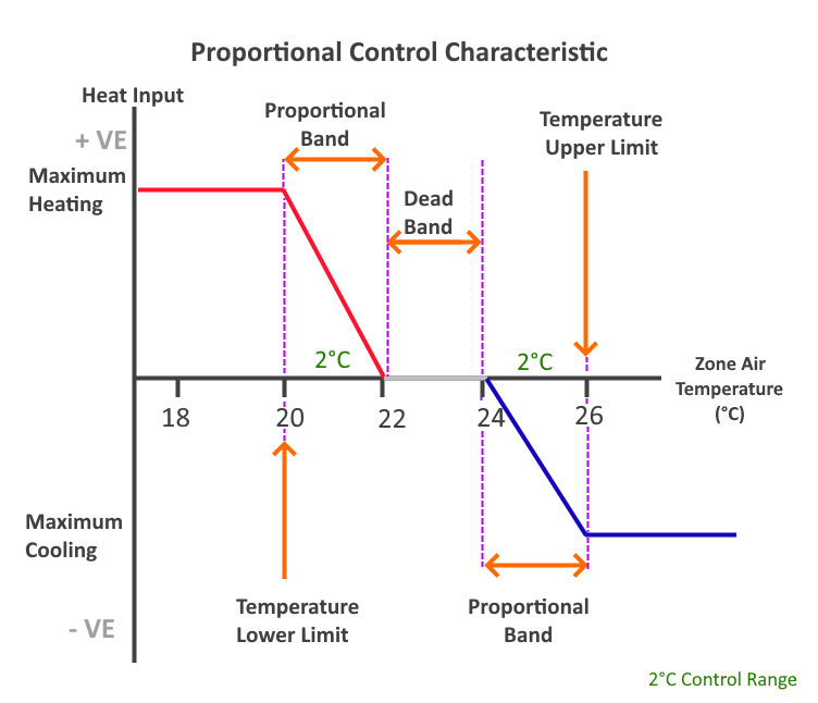
Proportional control
When the proportional control checkbox is disabled, the heating/cooling is either fully on or fully off, depending on the thermostat limits.
To model heating/cooling with a capacity that varies depending on a temperature range, check the proportional control box and enter a control range.
Note
When the heating or cooling capacities are set to Sizing, the proportional control band is automatically set to 0. This means that, at the sizing condition, the temperature is held at the Lower or Upper limit.
Example: Proportional Control
If the Upper Limit was set to 26°C and the Lower Limit was set to 20°C with a 2°C control band, the heating would be supplied at a maximum at or below 20°C and would reduce proportionally to 0 as the temperature rises to 22°C.
The cooling would be supplied at a maximum when the air temperature is above 26°C, and would reduce proportionally to 0 as the temperature reaches 24°C.
Between 22°C and 24°C, no heating or cooling would be supplied.
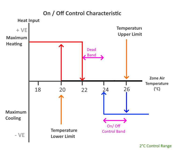
Example: On/Off Control
To model on/off control, uncheck the Proportional Control checkbox. If the control band is set to 2°C and the Upper Limit is 26°C with a Lower Limit of 24°C, the system will behave as follows.
Below 20°C, maximum heating is supplied. Above 26°C, maximum cooling is supplied. Between 22°C-24°C (dead band), there is no heating or cooling.
With this setup, there are two control bands- [20°C to 22°C] and [24°C to 26°C]. When the temperature is in one of these control bands, the amount of heating or cooling depends on the direction the band was entered.
If the air temperature enters the heating control band from below, the system supplies maximum heating until the temperature passes through the top of the band (22°C) and is switched off.
If the air temperature then falls back into the heating band, this time it is entering from above and the heating will remain off until the temperature passes through the lower limit of the band (20°C).
The same principle applies to the cooling band, and is illustrated in the diagram below:
System Parameters
The system parameters section of Internal Conditions used in Tas Systems and in the UK Building Regulations Studios.
Note
For UK Building regulations, NCM Internal Conditions should not be edited and this includes system parameters.
Metabolic Rate
Measured in Watts per Person, this field represents the amount of energy due to occupants transferred to the zone as heat.
The occupancy gains (sensible + latent) in \(W/m^2\) divided by the metabolic rate \(W/p\) will give the specified people density for the zone in \(p/m^2\).
DHW
Measured in litres per day per This field is used to calculate the domestic hot water load for Part L2 and EPCs.
Outside Air
Measured in litres per second per person, this field is used to determine the minimum fresh air requirement for part L2 and EPCs, and is also available in Tas Systems.
Target Room Illuminance
Measured in lux, this field is used to determine the required illuminance level within the zone at which the lighting gain will be set to its minimum. This field is primarily used in the UK Building regulations studio.
Profiles
Internal gains and thermostat gains can have different profiles depending on whether the gain being modelled is static in nature, or varies. The profile assigned to an internal gain / thermostat gain can be changed by clicking on the name of the gain:
The following window will appear, and the Type dropdown menu can be used to select the profile type:
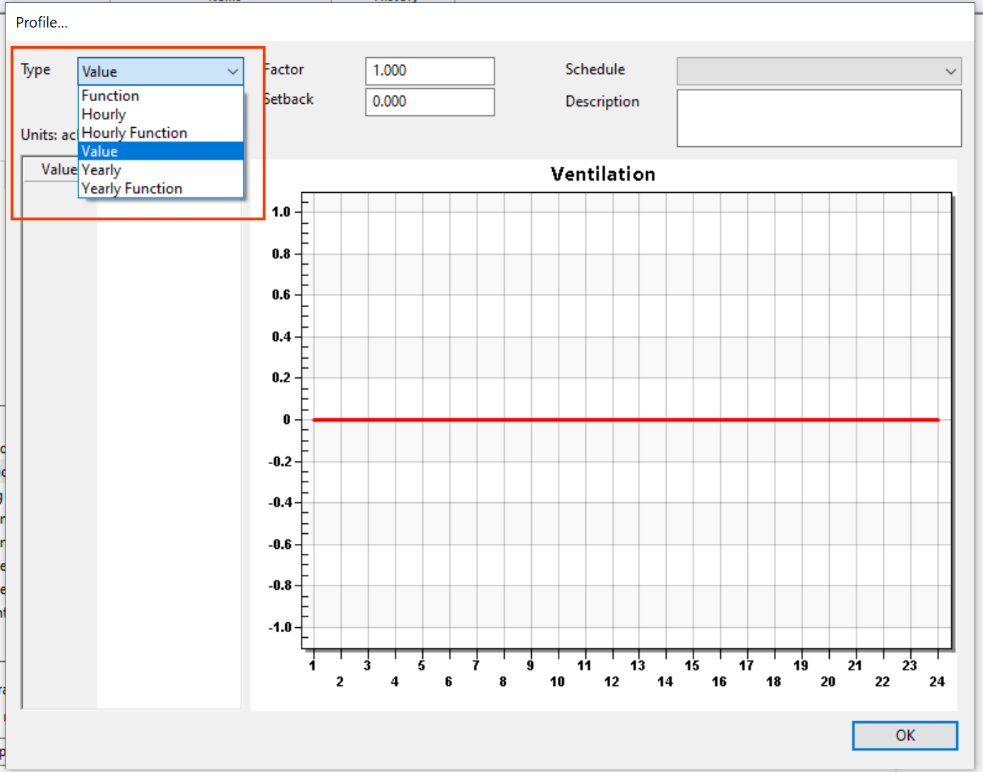
Gains can have the following profile types:
Value
Yearly
Hourly
Function
Hourly Function
Yearly Function
Not all types are available for all types of gain. For example, thermostat gains (e.g upper limit, lower limit) can only have the following types:
Hourly
Value
Yearly
Value
This is the default profile associated with an internal gain, and is used when the value is not expected to change and is expected to be constant. When this option is selected, the value of the profile is displayed in the internal condition tab:
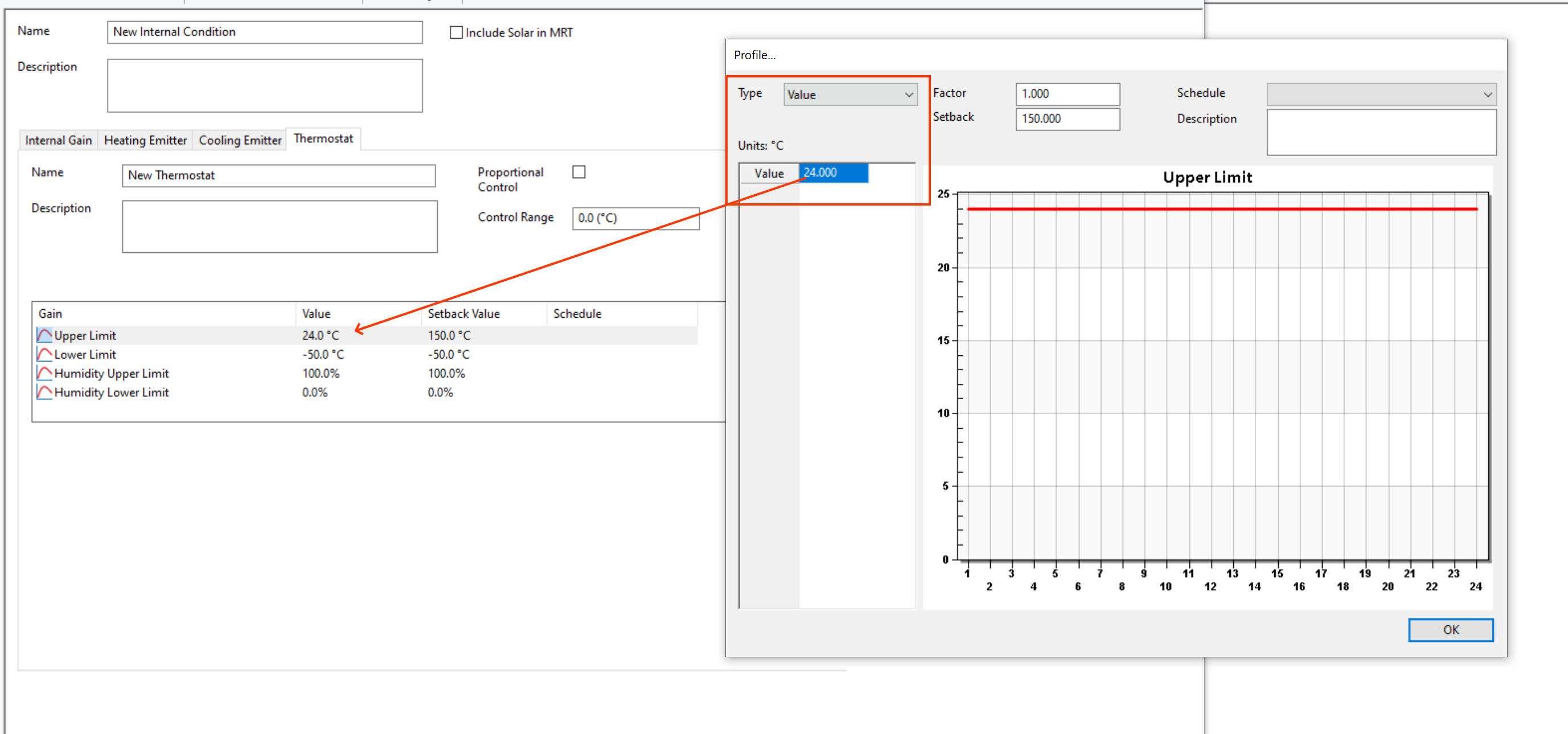
In the above example, the upper limit is set to 24°C. This means that zones that have this internal conditioned assigned will receive constant cooling to 24°C, if the internal condition applies to that day type.
This is also reflected in the graph, which shows a straight line. If this was combined with a schedule, the single value would apply during the scheduled hours. E.g., for a 9am-5pm schedule:
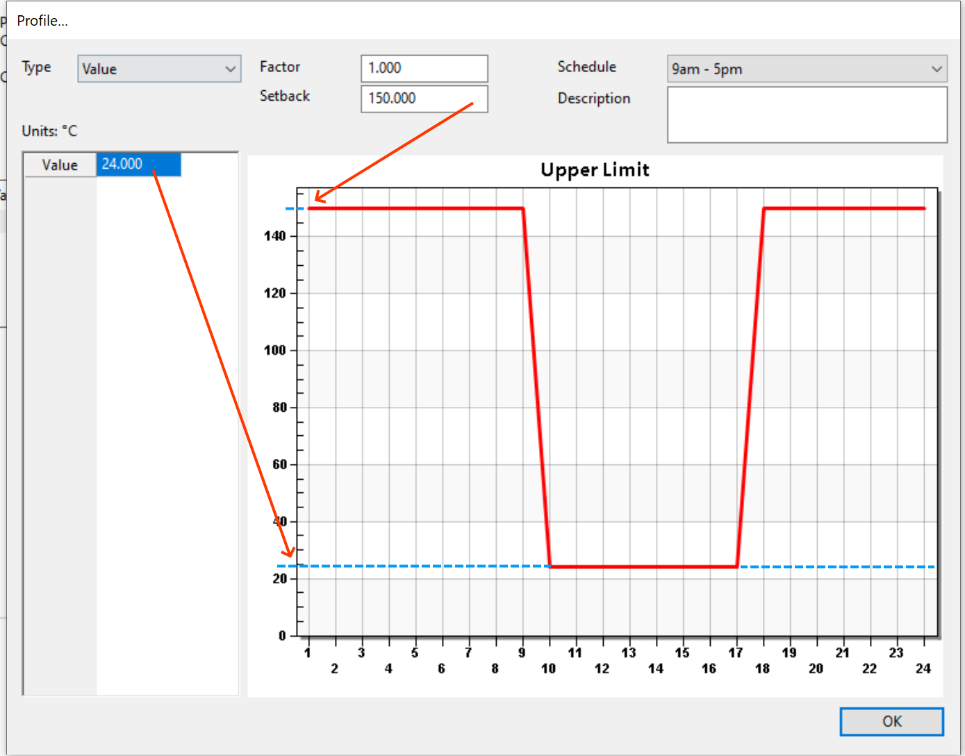
In the above image, we can see that the cooling is supplied to maintain 24°C according to the thermostat during the 9am-5pm period, but outside this period the setback value of 150°C (no cooling) is used.
Yearly
The Yearly Profile type is used to specify a value for the gain, for every hour of the year:
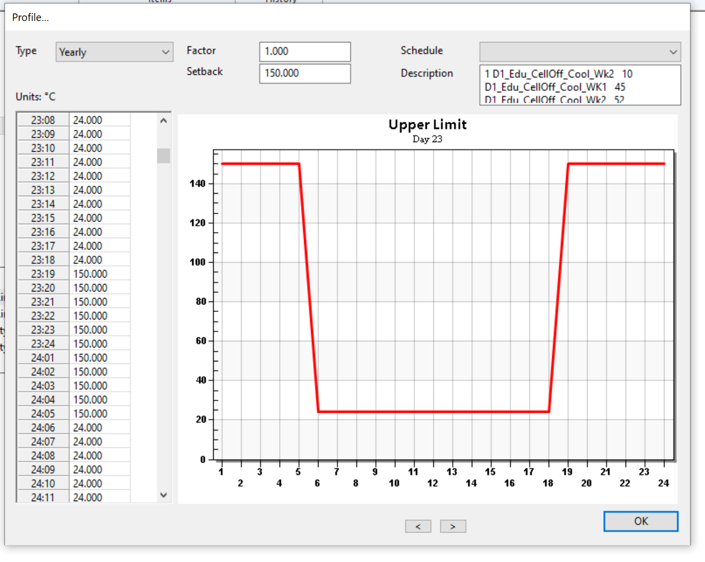
In the above, 23:18 means that on day 23 at hour 18, the gain has a value of 24°C. at 23:19, the gain has a value of 50°C.
If you assigned a schedule in conjunction with a yearly profile, the setback value would be used outside of the scheduled hours. This will be reflected in the graph.
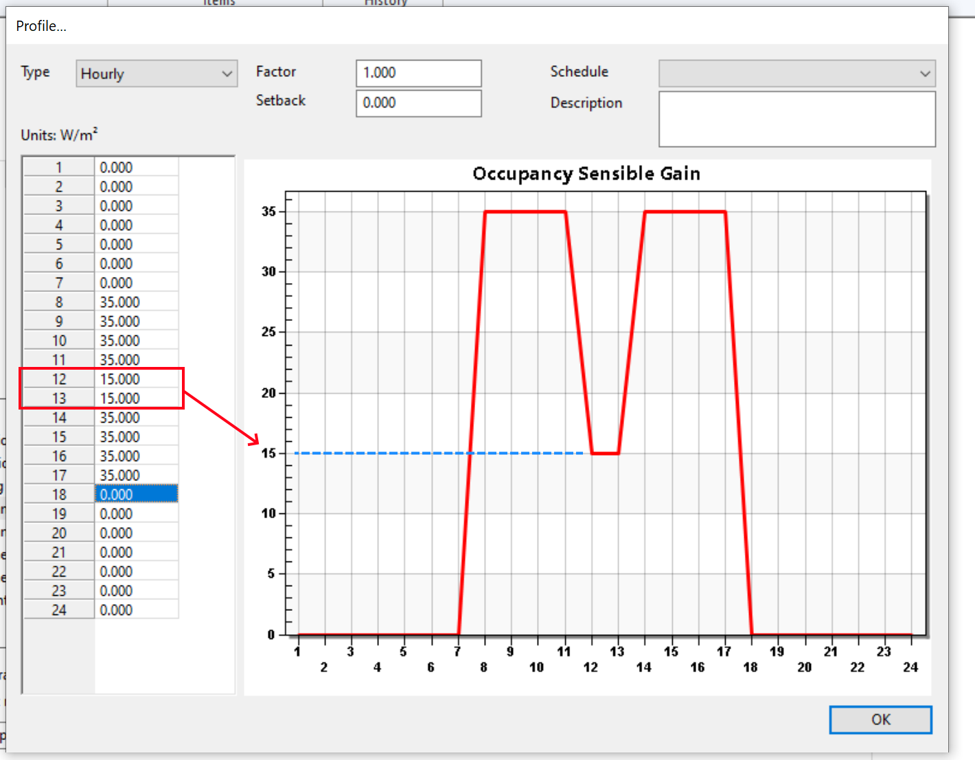
Hourly
The Hourly Profile type is similar to the Yearly Profile type, except 24 hourly values are assigned that are repeated for every day.
This is useful if you want to model reduced occupancy during a lunch break, for example:
Again, if a schedule is assigned then outside of the scheduled hours, the setback value will apply.
Function
The Function profile type is used to model gains that vary depending on some other parameters.
For example, if you wanted to vary the lighting gain based on the amount of natural illumination in a zone, you could use a lighting control function to model photocell control dimming.
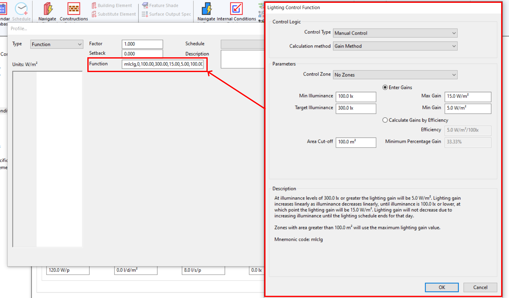
The function is actually a string, but when you select the function type, an editor pops up like the lighting editor shown above, to help write the function string for you.
For more information about lighting control functions and ventilation functions, see the relevant sections of the documentation.
Yearly Function
The Yearly Function type is very similar to the Function type, but it also allows you to specify a factor for every hour of the year. This factor is then multiplied by the value calculated by the function to calculate the gain.
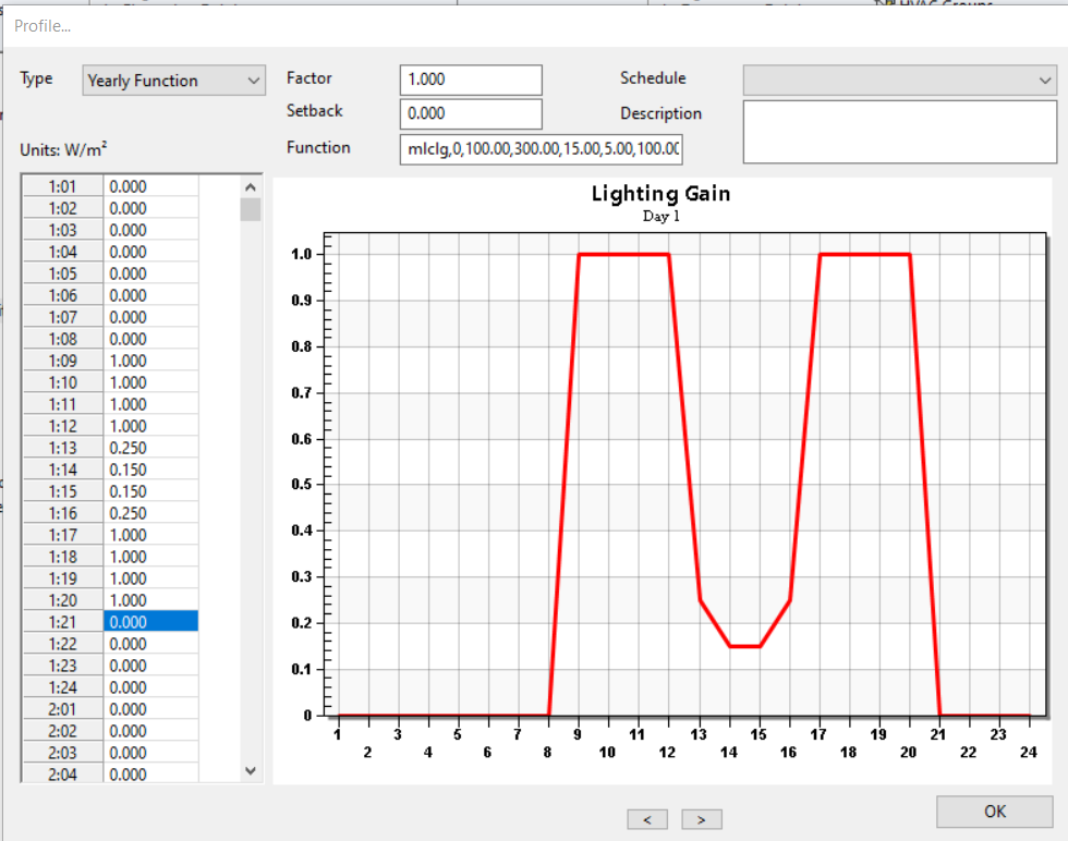
Schedules can be used in conjunction with yearly profiles; during “off” hours, the setback value will used.
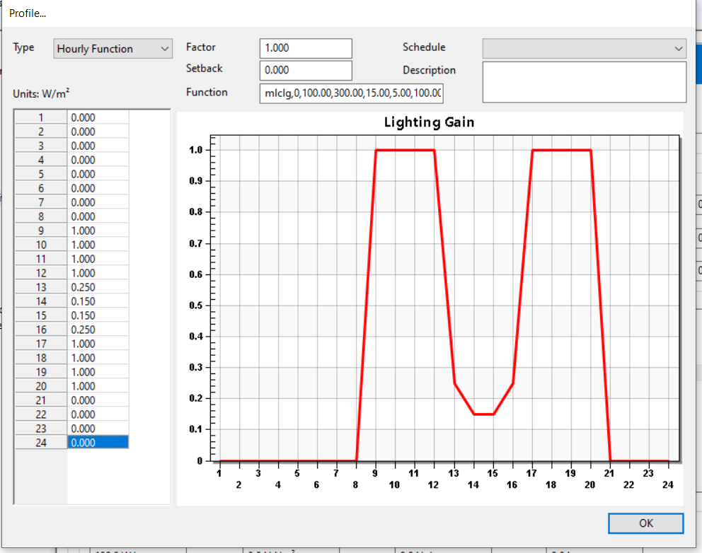
Hourly Function
The Hourly Function type is identical to the Yearly Function type, except 24 factors are specified representing a single day, which is then repeated for every hour of the simulation on the applied day types:
Again, schedules can be used in conjunction with yearly profiles; during “off” hours, the setback value will be used.